Eikonal traveltime tomography for seismic exploration scenarios
@Author: Ettore Biondi - ebiondi@caltech.edu
To use this notebook, we need pykonal installed. In your env, you can install it by:
conda install cythonpip install git+https://github.com/malcolmw/pykonal@0.2.3b3
In this notebook, we will apply the Eikonal tomography operators on a more realistic example using the Marmousi2 model. We will test two scenarios:
import numpy as np
import occamypy as o
import eikonal2d as k

# Plotting
from matplotlib import rcParams
from mpl_toolkits.axes_grid1 import make_axes_locatable
import matplotlib.pyplot as plt
rcParams.update({
    'image.cmap'     : 'jet',
    'image.aspect'   : 'equal',
    'axes.grid'      : True,
    'figure.figsize' : (19, 8),
    'savefig.dpi'    : 300,
    'axes.labelsize' : 14,
    'axes.titlesize' : 16,
    'font.size'      : 14,
    'legend.fontsize': 14,
    'xtick.labelsize': 14,
    'ytick.labelsize': 14,
})
WARNING! DATAPATH not found. The folder /tmp will be used to write binary files
/Library/Frameworks/Python.framework/Versions/3.9/lib/python3.9/site-packages/dask_jobqueue/core.py:20: FutureWarning: tmpfile is deprecated and will be removed in a future release. Please use dask.utils.tmpfile instead.
  from distributed.utils import tmpfile
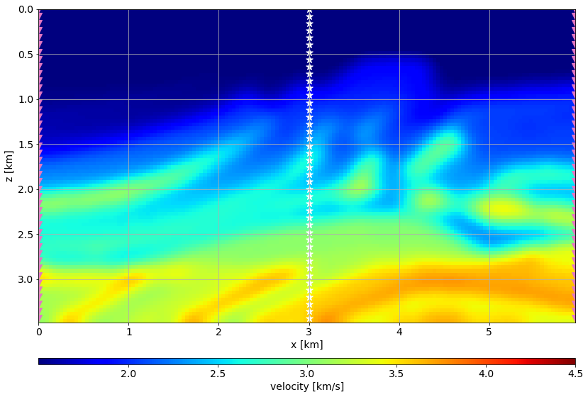
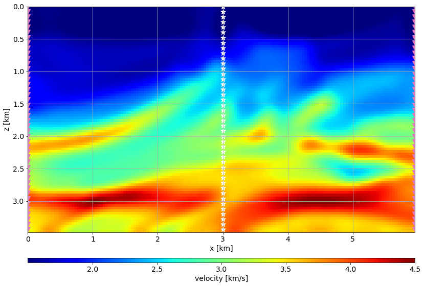
Cross-well tomography
Let's plot the true model. Along with the geometry for the cross-well tomography example using a section of the Marmousi.
# Reading velocity model
nx = 1700
nz = 350
dx = 0.01
dz = 0.01
ox = 0.0
oz = 0.0
MarmTrue = np.reshape(np.fromfile("data/Marmousi2Vp.bin", dtype=">f"), (nx,nz)).astype(np.float32)

MarmTrue = MarmTrue[600:1200,:]

desampling=4
dx *= desampling
dz *= desampling
MarmTrue = MarmTrue[::desampling,::desampling]
nx,nz = MarmTrue.shape

# Velocity model
vvTrue = o.VectorNumpy(MarmTrue, ax_info=[o.AxInfo(nx, ox, dx, "x [km]"),
                                          o.AxInfo(nz, oz, dz, "z [km]")])

extent = [vvTrue.ax_info[0].o, vvTrue.ax_info[0].last, vvTrue.ax_info[1].last, vvTrue.ax_info[1].o]
# Source/Receiver positions
SouPos = np.array([[int(nx*0.5),iz] for iz in np.arange(0,nz,2)])
RecPos = np.array([[0,iz] for iz in np.arange(0,nz,2)]+[[nx-1,iz] for iz in np.arange(0,nz,2)])fig, ax = plt.subplots()
im = ax.imshow(vvTrue.plot().T, extent=extent)
ax.scatter(SouPos[:,0]*dx, SouPos[:,1]*dz,color="white", marker="*", s=100)
ax.scatter(RecPos[:,0]*dx, RecPos[:,1]*dz, color="tab:pink", marker="v",s=100)
plt.xlabel(vvTrue.ax_info[0].l)
plt.ylabel(vvTrue.ax_info[1].l)
cbar = plt.colorbar(im, orientation="horizontal", label="velocity [km/s]",
cax=make_axes_locatable(ax).append_axes("bottom", size="2%", pad=0.7))
plt.tight_layout()
plt.show()---------------------------------------------------------------------------
NameError Traceback (most recent call last)
Input In [1], in <cell line: 1>()
----> 1 fig, ax = plt.subplots()
2 im = ax.imshow(vvTrue.plot().T, extent=extent)
4 ax.scatter(SouPos[:,0]*dx, SouPos[:,1]*dz,color="white", marker="*", s=100)
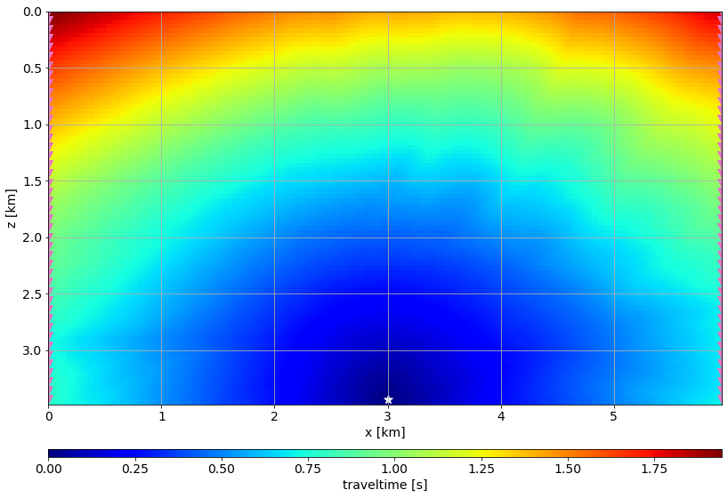
NameError: name 'plt' is not definedNow, we can proceed to generate the observed travel times.
# Data vector
tt_obs = o.VectorNumpy((SouPos.shape[0], RecPos.shape[0]),
                        ax_info=[o.AxInfo(SouPos.shape[0], 0, 1, "sou_id"),
                                 o.AxInfo(RecPos.shape[0], 0, 1, "rec_id")]).zero()

# Setting Forward non-linear operator
Eik2D_Op = k.EikonalTT_2D(vvTrue, tt_obs, SouPos, RecPos)
Eik2D_Op.forward(False, vvTrue, tt_obs)
sou_id = -1
fig, ax = plt.subplots()
im = ax.imshow(Eik2D_Op.tt_maps[sou_id].T, extent=extent)
ax.scatter(SouPos[sou_id,0]*dx,SouPos[sou_id,1]*dz,color="white", marker="*", s=100)
ax.scatter(RecPos[:,0]*dx, RecPos[:,1]*dz, color="tab:pink", marker="v",s=100)
plt.xlabel(vvTrue.ax_info[0].l)
plt.ylabel(vvTrue.ax_info[1].l)
cbar = plt.colorbar(im, orientation="horizontal", label="traveltime [s]",
cax=make_axes_locatable(ax).append_axes("bottom", size="2%", pad=0.7))
plt.tight_layout()
plt.show()/var/folders/q3/lmm60bhj01xcxkxyn8zc_mdm0000gn/T/ipykernel_99483/594416931.py:13: MatplotlibDeprecationWarning: Auto-removal of grids by pcolor() and pcolormesh() is deprecated since 3.5 and will be removed two minor releases later; please call grid(False) first.
cbar = plt.colorbar(im, orientation="horizontal", label="traveltime [s]",
# Plotting traveltime vector
fig, ax = plt.subplots(figsize=(10,4))
ax.plot(tt_obs.ax_info[1].plot(), tt_obs[0,:], lw=2)
ax.plot(tt_obs.ax_info[1].plot(), tt_obs[15,:], lw=2)
ax.plot(tt_obs.ax_info[1].plot(), tt_obs[-1,:], lw=2)

plt.xlabel(tt_obs.ax_info[1].l)
plt.ylabel("Traveltime [s]")

ax.set_ylim(tt_obs.max()+1.0, 0)
ax.set_xlim(tt_obs.ax_info[1].o, tt_obs.ax_info[1].last)

plt.tight_layout()
plt.show()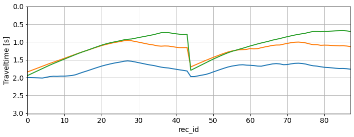
The initial model will be constructed by smoothing the true model.
G = o.GaussianFilter(vvTrue, 2.5)
vvInit = G * vvTrue
fig, ax = plt.subplots()
im = ax.imshow(vvInit.plot().T, extent=extent, vmin=vvTrue.min(), vmax=vvTrue.max())
ax.scatter(SouPos[:,0]*dx, SouPos[:,1]*dz,color="white", marker="*", s=100)
ax.scatter(RecPos[:,0]*dx, RecPos[:,1]*dz, color="tab:pink", marker="v",s=100)
plt.xlabel(vvTrue.ax_info[0].l)
plt.ylabel(vvTrue.ax_info[1].l)
cbar = plt.colorbar(im, orientation="horizontal", label="velocity [km/s]",
cax=make_axes_locatable(ax).append_axes("bottom", size="2%", pad=0.7))
plt.tight_layout()
plt.show()/var/folders/q3/lmm60bhj01xcxkxyn8zc_mdm0000gn/T/ipykernel_99483/1045714305.py:11: MatplotlibDeprecationWarning: Auto-removal of grids by pcolor() and pcolormesh() is deprecated since 3.5 and will be removed two minor releases later; please call grid(False) first.
cbar = plt.colorbar(im, orientation="horizontal", label="velocity [km/s]",
Let's set up the inversion problem and solve it.
# linear operator
Eik2D_Lin_Op = k.EikonalTT_lin_2D(vvInit, tt_obs, SouPos, RecPos, tt_maps=Eik2D_Op.tt_maps)

# nonlinear operator
Eik2D_NlOp = o.NonlinearOperator(Eik2D_Op, Eik2D_Lin_Op, Eik2D_Lin_Op.set_vel)
# instantiate solver
BFGSsolver = o.LBFGS(o.BasicStopper(niter=20, tolg_proj=1e-32), m_steps=30)
G = o.GaussianFilter(vvInit, 3.5)
Eik2D_Inv_NlOp = o.NonlinearOperator(Eik2D_Op, Eik2D_Lin_Op * G, Eik2D_Lin_Op.set_vel)
L2_tt_prob = o.NonlinearLeastSquares(vvInit.clone(), tt_obs, Eik2D_Inv_NlOp,
minBound=vvInit.clone().set(1.0), # min velocity: 1.0 km/s
maxBound=vvInit.clone().set(5.0)) # max velocity: 5.0 km/sBFGSsolver.run(L2_tt_prob, verbose=True)##########################################################################################
Limited-memory Broyden-Fletcher-Goldfarb-Shanno (L-BFGS) algorithm
Maximum number of steps to be used for Hessian inverse estimation: 30
Restart folder: /tmp/restart_2022-04-26T08-07-38.759082/
##########################################################################################
iter = 00, obj = 7.82079e+01, resnorm = 1.25e+01, gradnorm = 6.43e+00, feval = 1, geval = 1
iter = 01, obj = 1.56800e+01, resnorm = 5.60e+00, gradnorm = 1.23e+00, feval = 2, geval = 2
iter = 02, obj = 1.10747e+01, resnorm = 4.71e+00, gradnorm = 8.82e-01, feval = 3, geval = 3
iter = 03, obj = 5.34776e+00, resnorm = 3.27e+00, gradnorm = 6.37e-01, feval = 4, geval = 4
iter = 04, obj = 3.42891e+00, resnorm = 2.62e+00, gradnorm = 5.18e-01, feval = 5, geval = 5
iter = 05, obj = 1.88919e+00, resnorm = 1.94e+00, gradnorm = 3.14e-01, feval = 6, geval = 6
iter = 06, obj = 1.37063e+00, resnorm = 1.66e+00, gradnorm = 2.50e-01, feval = 7, geval = 7
iter = 07, obj = 1.01677e+00, resnorm = 1.43e+00, gradnorm = 2.25e-01, feval = 8, geval = 8
iter = 08, obj = 7.22148e-01, resnorm = 1.20e+00, gradnorm = 1.68e-01, feval = 9, geval = 9
iter = 09, obj = 5.91143e-01, resnorm = 1.09e+00, gradnorm = 1.22e-01, feval = 10, geval = 10
iter = 10, obj = 5.06263e-01, resnorm = 1.01e+00, gradnorm = 9.90e-02, feval = 11, geval = 11
iter = 11, obj = 4.42715e-01, resnorm = 9.41e-01, gradnorm = 8.93e-02, feval = 12, geval = 12
iter = 12, obj = 3.94955e-01, resnorm = 8.89e-01, gradnorm = 8.11e-02, feval = 13, geval = 13
iter = 13, obj = 3.55573e-01, resnorm = 8.43e-01, gradnorm = 7.14e-02, feval = 14, geval = 14
iter = 14, obj = 3.25080e-01, resnorm = 8.06e-01, gradnorm = 6.17e-02, feval = 15, geval = 15
iter = 15, obj = 3.03020e-01, resnorm = 7.78e-01, gradnorm = 5.27e-02, feval = 16, geval = 16
iter = 16, obj = 2.85325e-01, resnorm = 7.55e-01, gradnorm = 4.67e-02, feval = 17, geval = 17
iter = 17, obj = 2.68460e-01, resnorm = 7.33e-01, gradnorm = 4.52e-02, feval = 18, geval = 18
iter = 18, obj = 2.49967e-01, resnorm = 7.07e-01, gradnorm = 4.44e-02, feval = 19, geval = 19
iter = 19, obj = 2.33850e-01, resnorm = 6.84e-01, gradnorm = 3.87e-02, feval = 20, geval = 20
iter = 20, obj = 2.22291e-01, resnorm = 6.67e-01, gradnorm = 3.11e-02, feval = 21, geval = 21
Terminate: maximum number of iterations reached
##########################################################################################
Limited-memory Broyden-Fletcher-Goldfarb-Shanno (L-BFGS) algorithm end
##########################################################################################
fig, ax = plt.subplots()

im = ax.imshow(L2_tt_prob.model.plot().T, extent=extent, vmin=vvTrue.min(), vmax=vvTrue.max())

ax.scatter(SouPos[:,0]*dx, SouPos[:,1]*dz,color="white", marker="*", s=100)
ax.scatter(RecPos[:,0]*dx, RecPos[:,1]*dz, color="tab:pink", marker="v",s=100)

plt.xlabel(vvTrue.ax_info[0].l)
plt.ylabel(vvTrue.ax_info[1].l)

cbar = plt.colorbar(im, orientation="horizontal", label="velocity [km/s]",
                    cax=make_axes_locatable(ax).append_axes("bottom", size="2%", pad=0.7))

plt.tight_layout()
plt.show()
/var/folders/q3/lmm60bhj01xcxkxyn8zc_mdm0000gn/T/ipykernel_99483/3560037947.py:11: MatplotlibDeprecationWarning: Auto-removal of grids by pcolor() and pcolormesh() is deprecated since 3.5 and will be removed two minor releases later; please call grid(False) first.
cbar = plt.colorbar(im, orientation="horizontal", label="velocity [km/s]",
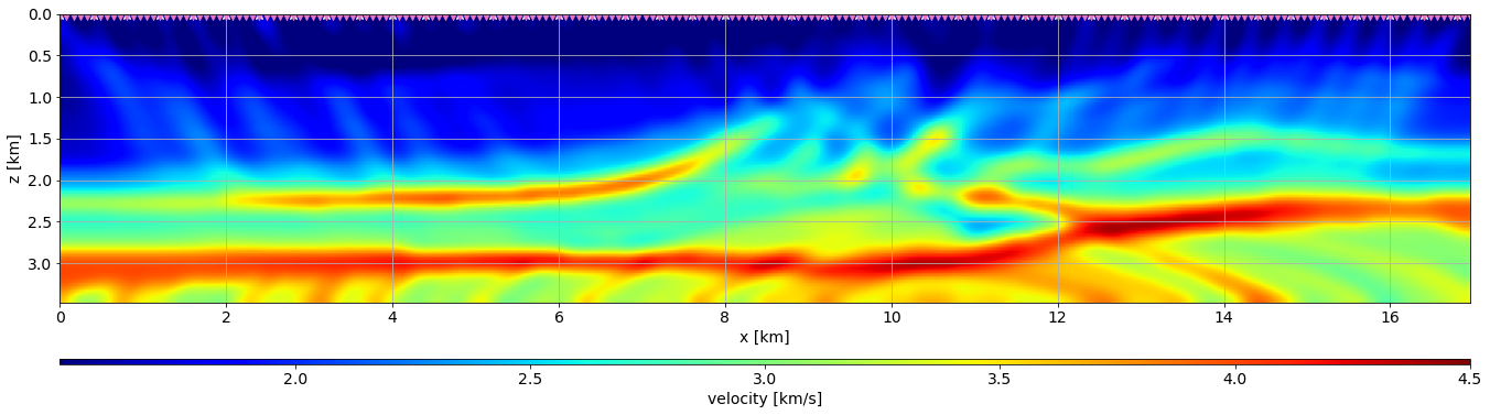
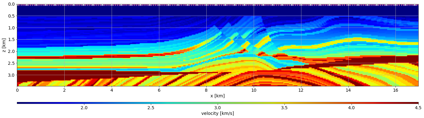
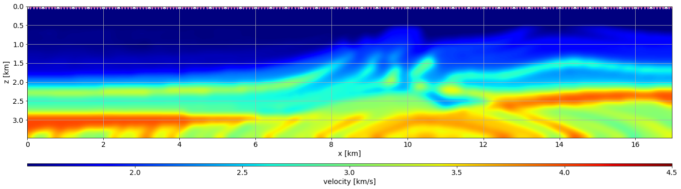
First-break surface tomography
In this test we will be estimating the subsurface velocity using a surface acquisition.
# Reading velocity model
nx = 1700
nz = 350
dx = 0.01
dz = 0.01
ox = 0.0
oz = 0.0
MarmTrue = np.reshape(np.fromfile("data/Marmousi2Vp.bin", dtype=">f"), (nx,nz)).astype(np.float32)

desampling=4
dx *= desampling
dz *= desampling
MarmTrue = MarmTrue[::desampling,::desampling]
nx,nz = MarmTrue.shape

# Velocity model
vvTrue = o.VectorNumpy(MarmTrue, ax_info=[o.AxInfo(nx, 0, dx, "x [km]"),
                                          o.AxInfo(nz, 0, dz, "z [km]")])

extent = [vvTrue.ax_info[0].o, vvTrue.ax_info[0].last, vvTrue.ax_info[1].last, vvTrue.ax_info[1].o]
# Source/Receiver positions
SouPos = np.array([[ix,0] for ix in np.arange(0,nx,10)])
RecPos = np.array([[ix,0] for ix in np.arange(0,nx,2)])fig, ax = plt.subplots()
im = ax.imshow(vvTrue.plot().T, extent=extent)
ax.scatter(RecPos[:,0]*dx, RecPos[:,1]*dz, color="tab:pink", marker="v",s=100)
ax.scatter(SouPos[:,0]*dx, SouPos[:,1]*dz,color="white", marker="*", s=100)
plt.xlabel(vvTrue.ax_info[0].l)
plt.ylabel(vvTrue.ax_info[1].l)
cbar = plt.colorbar(im, orientation="horizontal", label="velocity [km/s]",
cax=make_axes_locatable(ax).append_axes("bottom", size="2%", pad=0.7))
plt.tight_layout()
plt.show()/var/folders/q3/lmm60bhj01xcxkxyn8zc_mdm0000gn/T/ipykernel_99483/3681826258.py:11: MatplotlibDeprecationWarning: Auto-removal of grids by pcolor() and pcolormesh() is deprecated since 3.5 and will be removed two minor releases later; please call grid(False) first.
cbar = plt.colorbar(im, orientation="horizontal", label="velocity [km/s]",
# Data vector
tt_obs = o.VectorNumpy((SouPos.shape[0], RecPos.shape[0]),
ax_info=[o.AxInfo(SouPos.shape[0], 0, 1, "sou_id"),
o.AxInfo(RecPos.shape[0], 0, 1, "rec_id")]).zero()
# Setting Forward non-linear operator
Eik2D_Op = k.EikonalTT_2D(vvTrue, tt_obs, SouPos, RecPos)
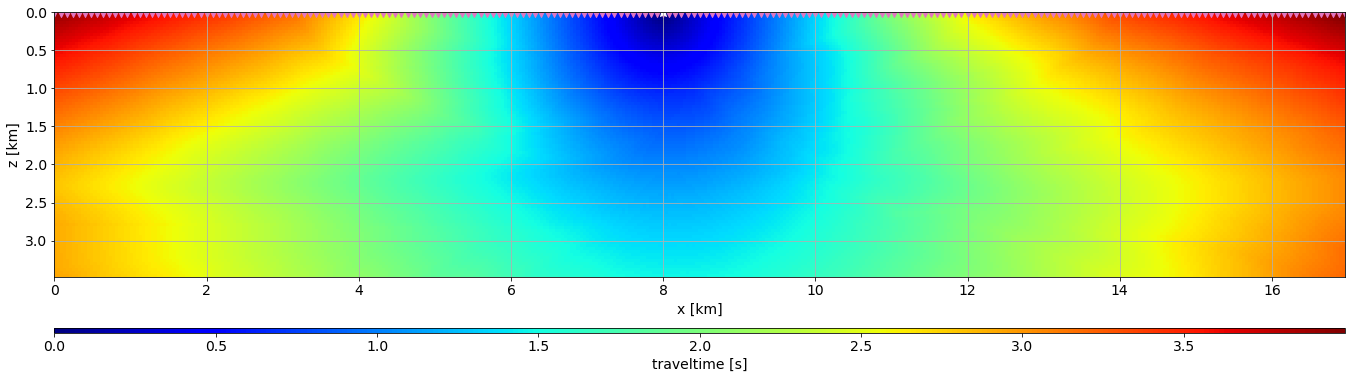
Eik2D_Op.forward(False, vvTrue, tt_obs)sou_id = 20
fig, ax = plt.subplots()
im = ax.imshow(Eik2D_Op.tt_maps[sou_id].T, extent=extent)
ax.scatter(RecPos[:,0]*dx, RecPos[:,1]*dz, color="tab:pink", marker="v",s=100)
ax.scatter(SouPos[sou_id,0]*dx, SouPos[sou_id,1]*dz, color="white", marker="*", s=100)
plt.xlabel(vvTrue.ax_info[0].l)
plt.ylabel(vvTrue.ax_info[1].l)
cbar = plt.colorbar(im, orientation="horizontal", label="traveltime [s]",
cax=make_axes_locatable(ax).append_axes("bottom", size="2%", pad=0.7))
plt.tight_layout()
plt.show()/var/folders/q3/lmm60bhj01xcxkxyn8zc_mdm0000gn/T/ipykernel_99483/2480074603.py:13: MatplotlibDeprecationWarning: Auto-removal of grids by pcolor() and pcolormesh() is deprecated since 3.5 and will be removed two minor releases later; please call grid(False) first.
cbar = plt.colorbar(im, orientation="horizontal", label="traveltime [s]",
# Plotting traveltime vector
fig, ax = plt.subplots(figsize=(10,4))
ax.plot(tt_obs.ax_info[1].plot(), tt_obs[0,:], lw=2)
ax.plot(tt_obs.ax_info[1].plot(), tt_obs[15,:], lw=2)
ax.plot(tt_obs.ax_info[1].plot(), tt_obs[-1,:], lw=2)

plt.xlabel(tt_obs.ax_info[1].l)
plt.ylabel("Traveltime [s]")

ax.set_ylim(tt_obs.max()+1.0, 0)
ax.set_xlim(tt_obs.ax_info[1].o, tt_obs.ax_info[1].last)

plt.tight_layout()
plt.show()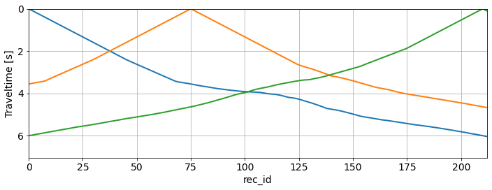
Again, let's create a initial smooth model
# Create Gaussian Filter
G = o.GaussianFilter(vvTrue, 2.5)
# Smoothing true model
vvInit = G * vvTrue
fig, ax = plt.subplots()
im = ax.imshow(vvInit.plot().T, extent=extent, vmin=vvTrue.min(), vmax=vvTrue.max())
ax.scatter(RecPos[:,0]*dx, RecPos[:,1]*dz, color="tab:pink", marker="v",s=100)
ax.scatter(SouPos[:,0]*dx, SouPos[:,1]*dz,color="white", marker="*", s=100)
plt.xlabel(vvTrue.ax_info[0].l)
plt.ylabel(vvTrue.ax_info[1].l)
cbar = plt.colorbar(im, orientation="horizontal", label="velocity [km/s]",
cax=make_axes_locatable(ax).append_axes("bottom", size="2%", pad=0.7))
plt.tight_layout()
plt.show()/var/folders/q3/lmm60bhj01xcxkxyn8zc_mdm0000gn/T/ipykernel_99483/995366468.py:11: MatplotlibDeprecationWarning: Auto-removal of grids by pcolor() and pcolormesh() is deprecated since 3.5 and will be removed two minor releases later; please call grid(False) first.
cbar = plt.colorbar(im, orientation="horizontal", label="velocity [km/s]",
# Linear operator
Eik2D_Lin_Op = k.EikonalTT_lin_2D(vvInit, tt_obs, SouPos, RecPos, tt_maps=Eik2D_Op.tt_maps)
# Nonlinear operator
Eik2D_NlOp = o.NonlinearOperator(Eik2D_Op, Eik2D_Lin_Op, Eik2D_Lin_Op.set_vel)
# Instantiate solver
BFGSsolver = o.LBFGS(o.BasicStopper(niter=20, tolg_proj=1e-32))
# Create non-linear operator
Eik2D_Inv_NlOp = o.NonlinearOperator(Eik2D_Op, Eik2D_Lin_Op * G, Eik2D_Lin_Op.set_vel)
L2_tt_prob = o.NonlinearLeastSquares(vvInit.clone(), tt_obs, Eik2D_Inv_NlOp,
minBound=vvInit.clone().set(1.0), # min velocity: 1.0 km/s
maxBound=vvInit.clone().set(5.0)) # max velocity: 5.0 km/sBFGSsolver.run(L2_tt_prob, verbose=True)##########################################################################################
Limited-memory Broyden-Fletcher-Goldfarb-Shanno (L-BFGS) algorithm
Maximum number of steps to be used for Hessian inverse estimation: 30
Restart folder: /tmp/restart_2022-04-26T08-09-13.204707/
##########################################################################################
iter = 00, obj = 1.21361e+03, resnorm = 4.93e+01, gradnorm = 5.51e+01, feval = 1, geval = 1
iter = 01, obj = 4.04259e+02, resnorm = 2.84e+01, gradnorm = 2.87e+01, feval = 2, geval = 2
iter = 02, obj = 7.41081e+01, resnorm = 1.22e+01, gradnorm = 7.51e+00, feval = 3, geval = 3
iter = 03, obj = 2.87076e+01, resnorm = 7.58e+00, gradnorm = 3.29e+00, feval = 4, geval = 4
iter = 04, obj = 1.76349e+01, resnorm = 5.94e+00, gradnorm = 2.29e+00, feval = 5, geval = 5
iter = 05, obj = 1.18068e+01, resnorm = 4.86e+00, gradnorm = 1.64e+00, feval = 6, geval = 6
iter = 06, obj = 8.80404e+00, resnorm = 4.20e+00, gradnorm = 1.13e+00, feval = 7, geval = 7
iter = 07, obj = 7.14773e+00, resnorm = 3.78e+00, gradnorm = 9.37e-01, feval = 8, geval = 8
iter = 08, obj = 6.16872e+00, resnorm = 3.51e+00, gradnorm = 8.93e-01, feval = 9, geval = 9
iter = 09, obj = 5.00490e+00, resnorm = 3.16e+00, gradnorm = 8.37e-01, feval = 10, geval = 10
iter = 10, obj = 4.05347e+00, resnorm = 2.85e+00, gradnorm = 7.59e-01, feval = 11, geval = 11
iter = 11, obj = 3.46407e+00, resnorm = 2.63e+00, gradnorm = 6.23e-01, feval = 12, geval = 12
iter = 12, obj = 2.90168e+00, resnorm = 2.41e+00, gradnorm = 5.89e-01, feval = 13, geval = 13
iter = 13, obj = 2.41457e+00, resnorm = 2.20e+00, gradnorm = 5.82e-01, feval = 14, geval = 14
iter = 14, obj = 1.96980e+00, resnorm = 1.98e+00, gradnorm = 4.94e-01, feval = 15, geval = 15
iter = 15, obj = 1.70803e+00, resnorm = 1.85e+00, gradnorm = 4.10e-01, feval = 16, geval = 16
iter = 16, obj = 1.51595e+00, resnorm = 1.74e+00, gradnorm = 3.63e-01, feval = 17, geval = 17
iter = 17, obj = 1.34359e+00, resnorm = 1.64e+00, gradnorm = 3.22e-01, feval = 18, geval = 18
iter = 18, obj = 1.20617e+00, resnorm = 1.55e+00, gradnorm = 2.71e-01, feval = 19, geval = 19
iter = 19, obj = 1.10572e+00, resnorm = 1.49e+00, gradnorm = 2.29e-01, feval = 20, geval = 20
iter = 20, obj = 1.03367e+00, resnorm = 1.44e+00, gradnorm = 2.01e-01, feval = 21, geval = 21
Terminate: maximum number of iterations reached
##########################################################################################
Limited-memory Broyden-Fletcher-Goldfarb-Shanno (L-BFGS) algorithm end
##########################################################################################
fig, ax = plt.subplots()

im = ax.imshow(L2_tt_prob.model.plot().T, extent=extent, vmin=vvTrue.min(), vmax=vvTrue.max())

ax.scatter(SouPos[:,0]*dx, SouPos[:,1]*dz,color="white", marker="*", s=100)
ax.scatter(RecPos[:,0]*dx, RecPos[:,1]*dz, color="tab:pink", marker="v",s=100)

plt.xlabel(vvTrue.ax_info[0].l)
plt.ylabel(vvTrue.ax_info[1].l)

cbar = plt.colorbar(im, orientation="horizontal", label="velocity [km/s]",
                    cax=make_axes_locatable(ax).append_axes("bottom", size="2%", pad=0.7))

plt.tight_layout()
plt.show()
/var/folders/q3/lmm60bhj01xcxkxyn8zc_mdm0000gn/T/ipykernel_99483/3560037947.py:11: MatplotlibDeprecationWarning: Auto-removal of grids by pcolor() and pcolormesh() is deprecated since 3.5 and will be removed two minor releases later; please call grid(False) first.
cbar = plt.colorbar(im, orientation="horizontal", label="velocity [km/s]",