Using PyLops and OccamyPy together
@Author: Francesco Picetti - picettifrancesco@gmail.com
In this notebook, we will combine PyLops and OccamyPy.
First, let me express my gratitude to Matteo Ravasi; PyLops has strongly inspired us to publish OccamyPy, as our contribution to the scientific community.
In the following, we leverage PyLops rich library of operators to be used with OccamyPy, which we found to be agile for distributed computation and nonlinear problems.
import numpy as np
import occamypy as o
import matplotlib.pyplot as plt
import pylops
WARNING! DATAPATH not found. The folder /tmp will be used to write binary files
/nas/home/fpicetti/miniconda3/envs/occd/lib/python3.10/site-packages/dask_jobqueue/core.py:20: FutureWarning: tmpfile is deprecated and will be removed in a future release. Please use dask.utils.tmpfile instead.
  from distributed.utils import tmpfile
Mechanism of the interface
Let's say we have a VectorNumpy
x = o.VectorNumpy((3,5)).set(1.)and we want to use a PyLops operator like
Dp = pylops.Diagonal(np.arange(x.size))we can cast such operator to OccamyPy with FromPylops
D = o.pylops_interface.FromPylops(domain=x, range=x, op=Dp)Now we have a OccamyPy operator that can be used in our inversion
D.dotTest(True)Dot-product tests of forward and adjoint operators
--------------------------------------------------
Applying forward operator add=False
Runs in: 3.24249267578125e-05 seconds
Applying adjoint operator add=False
Runs in: 1.5735626220703125e-05 seconds
Dot products add=False: domain=1.117678e+01 range=1.117678e+01
Absolute error: 0.000000e+00
Relative error: 0.000000e+00
Applying forward operator add=True
Runs in: 1.049041748046875e-05 seconds
Applying adjoint operator add=True
Runs in: 9.298324584960938e-06 seconds
Dot products add=True: domain=2.235356e+01 range=2.235356e+01
Absolute error: 0.000000e+00
Relative error: 0.000000e+00
-------------------------------------------------
At the same time, we can cast a Numpy-based OccamyPy operator to PyLops with ToPylops
S = o.Scaling(x, 2.)Sp = o.pylops_interface.ToPylops(S)Such operator can be used inside PyLops
pylops.utils.dottest(Sp, x.size, x.size, tol=1e-6, complexflag=0, verb=True)

print("\t", np.isclose((Sp * x.arr.ravel()).reshape(x.shape), 2. * x.arr).all())
Dot test passed, v^T(Opu)=-2.696536 - u^T(Op^Tv)=-2.696536
True
Example 1: CT Scan Imaging
Let's replicate this example. The modeling equation is
def radoncurve(x, r, theta):
    curve = (r - ny // 2) / (np.sin(np.deg2rad(theta)) + 1e-15) \
            + np.tan(np.deg2rad(90 - theta)) * x + ny // 2
    return curve
Load the image and create the 2D Radon transform operator as done in PyLops
x = np.load('data/shepp_logan_phantom.npy').T
x = x / x.max()
nx, ny = x.shape

ntheta = 150
theta = np.linspace(0., 180., ntheta, endpoint=False)

RLop = pylops.signalprocessing.Radon2D(np.arange(ny), np.arange(nx),
                                       theta, kind=radoncurve,
                                       centeredh=True, interp=False,
                                       engine='numpy', dtype='float64')
Let's see the operator at work
y = RLop.H * x.ravel()
y = y.reshape(ntheta, ny)

xrec = RLop * y.ravel()
xrec = xrec.reshape(nx, ny)

fig, axs = plt.subplots(1, 3, figsize=(10, 4))
axs[0].imshow(x.T, vmin=0, vmax=1, cmap='gray')
axs[0].set_title('Model')
axs[0].axis('tight')
axs[1].imshow(y.T, cmap='gray')
axs[1].set_title('Data')
axs[1].axis('tight')
axs[2].imshow(xrec.T, cmap='gray')
axs[2].set_title('Adjoint domain')
axs[2].axis('tight')
fig.tight_layout()
plt.show()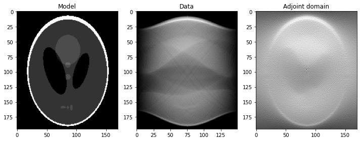
Now let's build the OccamyPy equivalent
x_ = o.VectorNumpy(x)
y_ = o.VectorNumpy((ntheta, ny))
R_ = o.pylops_interface.FromPylops(x_, y_, RLop.H)
y_ = R_ * x_
xrec_ = R_.H * y_
fig, axs = plt.subplots(1, 3, figsize=(10, 4))
axs[0].imshow(x_.plot().T, vmin=0, vmax=1, cmap='gray')
axs[0].set_title('Model')
axs[0].axis('tight')
axs[1].imshow(y_.plot().T, cmap='gray')
axs[1].set_title('Data')
axs[1].axis('tight')
axs[2].imshow(xrec_.plot().T, cmap='gray')
axs[2].set_title('Adjoint domain')
axs[2].axis('tight')
fig.tight_layout()
plt.show()Set up the TV-regularized inversion as done in PyLops
mu = 1.5
lamda = 1.
niter = 3
niterinner = 4

problemTV = o.GeneralizedLasso(x_.clone().zero(), y_, R_, eps=lamda / mu,
                               reg=o.Gradient(x_, stencil="backward"))

SB = o.SplitBregman(o.BasicStopper(niter=niter),
                    niter_inner=niterinner,
                    niter_solver=20,
                    linear_solver="LSQR",
                    warm_start=True)

SB.setDefaults(save_obj=True)
SB.run(problemTV, verbose=True, inner_verbose=False)##########################################################################################
SPLIT-BREGMAN Solver
Restart folder: /tmp/restart_2022-04-22T01-48-19.749447/
Inner iterations: 4
Solver iterations: 20
L1 Regularizer weight: 6.67e-01
Bregman update weight: 1.00e+00
Using warm start option for inner problem
##########################################################################################
iter = 0, obj = 5.43461e+06, df_obj = 5.43e+06, reg_obj = 0.00e+00, rnorm = 3.30e+03
iter = 1, obj = 1.58628e+03, df_obj = 2.20e+01, reg_obj = 1.56e+03, rnorm = 2.20e+01
iter = 2, obj = 1.41801e+03, df_obj = 1.39e+01, reg_obj = 1.40e+03, rnorm = 2.14e+01
iter = 3, obj = 1.26275e+03, df_obj = 1.44e+01, reg_obj = 1.25e+03, rnorm = 2.14e+01
Terminate: maximum number of iterations reached
##########################################################################################
SPLIT-BREGMAN Solver end
##########################################################################################
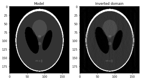
fig, axs = plt.subplots(1, 2, figsize=(7, 4))
axs[0].imshow(x_.plot().T, vmin=0, vmax=1, cmap='gray')
axs[0].set_title('Model')
axs[0].axis('tight')
axs[1].imshow(problemTV.model.plot().T, vmin=0, vmax=1, cmap='gray')
axs[1].set_title('Inverted domain')
axs[1].axis('tight')
fig.tight_layout()
plt.show()