The Split-Bregman Algorithm: Sparsity Enforcing Inversions
@Author: Francesco Picetti - picettifrancesco@gmail.com
In this notebook we will show the Split-Bregman algorithm, as described by Goldstein and Osher, 2009.
In its generalized unconstrained formulation (the same we handle in this library), this algorithm
takes what we call GeneralizedLasso (see occamypy.problem module):
being our model, the observed data, a linear modeling operator, the sparsity promoting regularizer and its weight .
Import modules
# Importing necessary modules
import numpy as np
import occamypy as o

# Plotting
from matplotlib import rcParams
from mpl_toolkits.axes_grid1 import make_axes_locatable
import matplotlib.pyplot as plt
rcParams.update({
    'image.cmap'     : 'gray',
    'image.aspect'   : 'auto',
    'image.interpolation': None,
    'axes.grid'      : True,
    'figure.figsize' : (12, 3),
    'savefig.dpi'    : 300,
    'axes.labelsize' : 14,
    'axes.titlesize' : 16,
    'font.size'      : 14,
    'legend.fontsize': 14,
    'xtick.labelsize': 14,
    'ytick.labelsize': 14,
    'text.usetex'    : True,
    'font.family'    : 'serif',
    'font.serif'     : 'Latin Modern Roman',
})
WARNING! DATAPATH not found. The folder /tmp will be used to write binary files
/Users/francesco/miniconda3/envs/swung/lib/python3.10/site-packages/dask_jobqueue/core.py:20: FutureWarning: tmpfile is deprecated and will be removed in a future release. Please use dask.utils.tmpfile instead.
  from distributed.utils import tmpfile
Example 1: 1D Ricker Deconvolution
In this example we want to invert a 1D seismic trace for the Earth's reflectivity. We suppose the wavelet to be known, yielding to a deterministic deconvolution problem.
# load wavelet
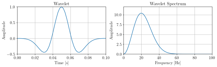
wav = o.VectorNumpy(np.load("./data/ricker20.npy"), ax_info=[o.AxInfo(n=51, o=0., d=0.002, l="time [s]")])
# load reflectivity
x = o.VectorNumpy(np.load("./data/reflectivity1D.npy"), ax_info=[o.AxInfo(n=1000, o=0., d=0.002, l="time [s]")])
# instantating operator
W = o.ConvND(x, wav)
# Generating true recorded trace
d = W * x
# Compute spectra
nfft = 4096
x_spectra = np.fft.fft(x.getNdArray(), nfft)
d_spectra = np.fft.fft(d.getNdArray(), nfft)
w_spectra = np.fft.fft(wav.getNdArray(), nfft)
freq = np.fft.fftfreq(nfft, wav.ax_info[0].d)time_axis = x.ax_info[0].plot()
xlim = x.ax_info[0].o, x.ax_info[0].last
xlbl = x.ax_info[0].lfig, ax = plt.subplots()
plt.plot(freq[:nfft//4], np.abs(x_spectra)[:nfft//4], 'k', label='model')
plt.plot(freq[:nfft//4], np.abs(d_spectra)[:nfft//4], 'b', label='data')
plt.legend(loc='upper right')
plt.xlabel("Frequency [Hz]"), plt.ylabel("Amplitude")
plt.xlim(0,100), plt.ylim(0,30)
plt.tight_layout(pad=0.5)
plt.show()
fig, ax = plt.subplots(1,2)
ax[0].plot(wav.ax_info[0].plot(), wav.plot())
ax[0].set_title('Wavelet')
ax[0].set_xlabel("Time [s]"), ax[0].set_ylabel("Amplitude")
ax[0].set_xlim(0,0.1), ax[0].set_ylim(-0.5,1)
ax[1].plot(freq[:nfft//4], np.abs(w_spectra)[:nfft//4])
ax[1].set_title('Wavelet Spectrum')
ax[1].set_xlabel("Frequency [Hz]"), ax[1].set_ylabel("Amplitude")
ax[1].set_xlim(0,100), ax[1].set_ylim(0,12)
plt.show()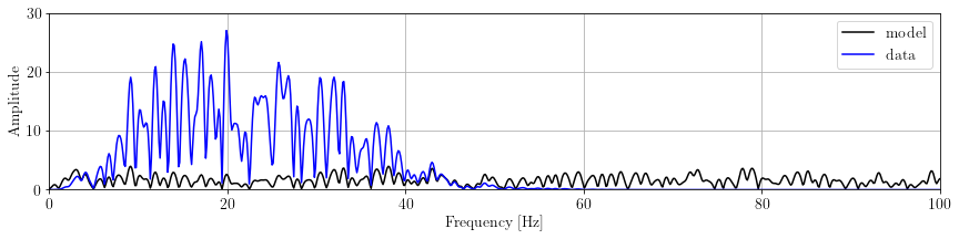
fig, ax = plt.subplots()
ax.plot(time_axis, x.plot(), 'k',  label='model')
ax.plot(time_axis, d.plot(), 'b',  label='data')
ax.legend(loc='upper left')
ax.set_ylim(-1., 1.), ax.set_xlim(*xlim)
ax.set_xlabel(xlbl), ax.set_ylabel("Amplitude")

axins1 = ax.inset_axes([0.42, 0.55, 0.1, 0.4])
axins1.plot(time_axis, x.plot(), 'k')
axins1.plot(time_axis, d.plot(), 'b')
axins1.set_xlim(0.76, 0.8)
axins1.set_ylim(-.1, .1)
axins1.set_xticklabels('')
axins1.set_yticklabels('')
ax.indicate_inset_zoom(axins1)

axins2 = ax.inset_axes([0.55, 0.55, 0.1, 0.4])
axins2.plot(time_axis, x.plot(), 'k')
axins2.plot(time_axis, d.plot(), 'b')
axins2.set_xlim(1.51, 1.59)
axins2.set_ylim(-.1, .1)
axins2.set_xticklabels('')
axins2.set_yticklabels('')
ax.indicate_inset_zoom(axins2)

axins3 = ax.inset_axes([0.49, 0.05, 0.1, 0.4])
axins3.plot(time_axis, x.plot(), 'k')
axins3.plot(time_axis, d.plot(), 'b')
axins3.set_xlim(1.0, 1.2)
axins3.set_ylim(-.1, .1)
axins3.set_xticklabels('')
axins3.set_yticklabels('')
ax.indicate_inset_zoom(axins3)

plt.suptitle("Model and Data")
plt.show()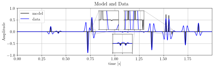
Solve with Conjugate Gradient
Conjugate gradient is a fast and powerful adjoint-state algorithm for solving problems in the form:
# instantiate a linear L2 problem
problemCG = o.LeastSquares(x.clone().zero(), d, W)

# define the solver with 10'000 iterations
CG = o.CG(o.BasicStopper(10000))
CG.setDefaults(save_obj=True)

# solve the problem
CG.run(problemCG, verbose=False)
fig, ax = plt.subplots()
ax.plot(time_axis, x.plot(), 'b', lw=2, label='true model')
ax.plot(time_axis, problemCG.model.plot(), 'r', label='CG')
ax.legend(loc='upper left')
ax.set_ylim(-1., 1.), ax.set_xlim(*xlim)
ax.set_xlabel(xlbl), ax.set_ylabel("Amplitude")
axins1 = ax.inset_axes([0.42, 0.55, 0.1, 0.4])
axins1.plot(time_axis, x.plot(), 'b', lw=2)
axins1.plot(time_axis, problemCG.model.plot(), 'r')
axins1.set_xlim(0.76, 0.8)
axins1.set_ylim(-.1, .1)
axins1.set_xticklabels('')
axins1.set_yticklabels('')
ax.indicate_inset_zoom(axins1)
axins2 = ax.inset_axes([0.55, 0.55, 0.1, 0.4])
axins2.plot(time_axis, x.plot(), 'b', lw=2)
axins2.plot(time_axis, problemCG.model.plot(), 'r')
axins2.set_xlim(1.51, 1.59)
axins2.set_ylim(-.1, .1)
axins2.set_xticklabels('')
axins2.set_yticklabels('')
ax.indicate_inset_zoom(axins2)
axins3 = ax.inset_axes([0.49, 0.05, 0.1, 0.4])
axins3.plot(time_axis, x.plot(), 'b', lw=2)
axins3.plot(time_axis, problemCG.model.plot(), 'r')
axins3.set_xlim(1.0, 1.2)
axins3.set_ylim(-.1, .1)
axins3.set_xticklabels('')
axins3.set_yticklabels('')
ax.indicate_inset_zoom(axins3)
plt.suptitle('Conjugate Gradient, %d it' % len(CG.obj))
plt.show()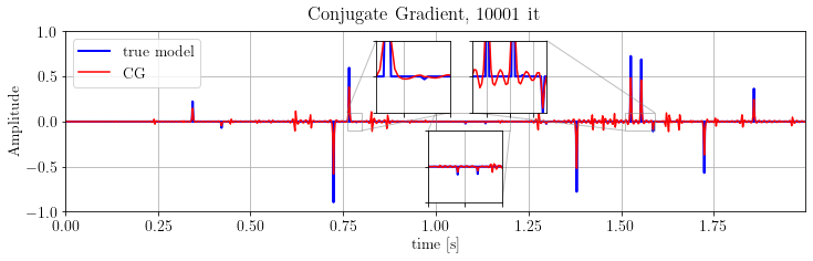
Impose sparsity in the solution: FISTA
Iterative Shrinkage-Thresholding Algorithms solve the so-called LASSO problem:
If we provide the operator's maximum eigenvalue we can build a fast version of this algorithm by imposing the step as proposed in Beck and Teboulle, 2009.
compute maximum eigenvalue
maxeig = W.powerMethod()
print('FISTA α=%.6e' % (1/(maxeig**2)))
FISTA α=9.288532e-03
# define the LASSO problem
problemFISTA = o.Lasso(x.clone().zero(), d, W, lambda_value=1, op_norm=maxeig**2)

# instantiate the fast solver with 1000 iterations
FISTA = o.ISTA(o.BasicStopper(10000), fast=True)
FISTA.setDefaults(save_obj=True)

# solve the problem
FISTA.run(problemFISTA, verbose=False)
fig, ax = plt.subplots()
ax.plot(time_axis, x.plot(), 'b', lw=2, label='true model')
ax.plot(time_axis, problemFISTA.model.plot(), 'r', label='FISTA')
ax.legend(loc='upper left')
ax.set_ylim(-1., 1.), ax.set_xlim(*xlim)
ax.set_xlabel(xlbl), ax.set_ylabel("Amplitude")
axins1 = ax.inset_axes([0.42, 0.55, 0.1, 0.4])
axins1.plot(time_axis, x.plot(), 'b', lw=2)
axins1.plot(time_axis, problemFISTA.model.plot(), 'r')
axins1.set_xlim(0.76, 0.8)
axins1.set_ylim(-.1, .1)
axins1.set_xticklabels('')
axins1.set_yticklabels('')
ax.indicate_inset_zoom(axins1)
axins2 = ax.inset_axes([0.55, 0.55, 0.1, 0.4])
axins2.plot(time_axis, x.plot(), 'b', lw=2)
axins2.plot(time_axis, problemFISTA.model.plot(), 'r')
axins2.set_xlim(1.51, 1.59)
axins2.set_ylim(-.1, .1)
axins2.set_xticklabels('')
axins2.set_yticklabels('')
ax.indicate_inset_zoom(axins2)
axins3 = ax.inset_axes([0.49, 0.05, 0.1, 0.4])
axins3.plot(time_axis, x.plot(), 'b', lw=2)
axins3.plot(time_axis, problemFISTA.model.plot(), 'r')
axins3.set_xlim(1.0, 1.2)
axins3.set_ylim(-.1, .1)
axins3.set_xticklabels('')
axins3.set_yticklabels('')
ax.indicate_inset_zoom(axins3)
plt.suptitle(r'Fast-ISTA, $\lambda=$%.e, %d it' % (problemFISTA.lambda_value, len(FISTA.obj)))
plt.show()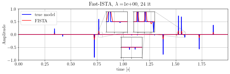
Note that FISTA is able to recover the model's kinematics but not the true amplitude. Indeed, this algorithm is very sensitive to parameter. Let's try another solver.
Split-Bregman for LASSO problem
# define the Linear Regularized Problem
problemSB = o.GeneralizedLasso(x.clone().zero(), d, W, reg=o.Identity(x), eps=.1)

# instantiate the Split-Bregman solver
SB = o.SplitBregman(o.BasicStopper(1000), niter_inner=3, niter_solver=5,
                    linear_solver='LSQR', breg_weight=1., warm_start=True)
SB.setDefaults(save_obj=True)
# solve the problem
SB.run(problemSB, verbose=False, inner_verbose=False)
its = "%d-%d-%d" % (len(SB.obj), SB.niter_inner, SB.niter_solver)fig, ax = plt.subplots()
ax.plot(time_axis, x.plot(), 'b', lw=2, label='true model')
ax.plot(time_axis, problemSB.model.plot(), 'r', label='SB')
ax.legend(loc='upper left')
ax.set_ylim(-1., 1.), ax.set_xlim(*xlim)
ax.set_xlabel(xlbl), ax.set_ylabel("Amplitude")
axins1 = ax.inset_axes([0.42, 0.55, 0.1, 0.4])
axins1.plot(time_axis, x.plot(), 'b', lw=2)
axins1.plot(time_axis, problemSB.model.plot(), 'r')
axins1.set_xlim(0.76, 0.8)
axins1.set_ylim(-.1, .1)
axins1.set_xticklabels('')
axins1.set_yticklabels('')
ax.indicate_inset_zoom(axins1)
axins2 = ax.inset_axes([0.55, 0.55, 0.1, 0.4])
axins2.plot(time_axis, x.plot(), 'b', lw=2)
axins2.plot(time_axis, problemSB.model.plot(), 'r')
axins2.set_xlim(1.51, 1.59)
axins2.set_ylim(-.1, .1)
axins2.set_xticklabels('')
axins2.set_yticklabels('')
ax.indicate_inset_zoom(axins2)
axins3 = ax.inset_axes([0.49, 0.05, 0.1, 0.4])
axins3.plot(time_axis, x.plot(), 'b', lw=2)
axins3.plot(time_axis, problemSB.model.plot(), 'r')
axins3.set_xlim(1.0, 1.2)
axins3.set_ylim(-.1, .1)
axins3.set_xticklabels('')
axins3.set_yticklabels('')
ax.indicate_inset_zoom(axins3)
plt.suptitle(r'Split-Bregman %s, $\varepsilon=%.e$' % (its, problemSB.eps))
plt.show()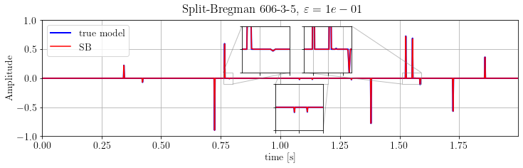
fig, ax = plt.subplots()
ax.semilogy(time_axis, np.abs(x.plot()), 'b', label="true model")
ax.semilogy(time_axis, np.abs(problemSB.model.plot()), 'r', label="SB")
ax.set_xlim(*xlim), ax.set_ylim(1e-8, 1)
ax.legend(loc='upper left')
ax.set_xlabel(xlbl), ax.set_ylabel("Amplitude")

plt.suptitle(r'Split-Bregman %s, $\varepsilon=%.e$' % (its, problemSB.eps))
plt.show()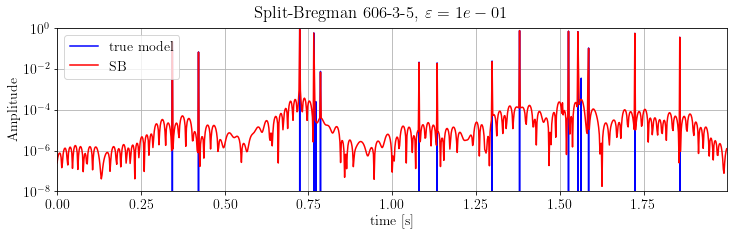
The results is much better than FISTA output: the dynamics is almost-perfectly recovered.
Example 2: 1D Velocity Deconvolution
Now we create a synthetic velocity profile and suppose to have recorded a smooth version of it. The deconvolution problem aims at recovering the sharp model, and this is done by using a Total Variation regularizer.
# create the true model
nx = 201
x = o.VectorNumpy((nx,), ax_info=[o.AxInfo(201, 0, 1, "depth [sample]")]).zero()
x[20:30] = 10.
x[50:75] = -5.
x[100:150] = 2.5
x[175:180] = 7.5

# instantiate the blurring operator
G = o.GaussianFilter(x, (2.,))

# simulate data
d = G * x
fig, ax = plt.subplots()
ax.plot(x.plot(), 'k', label='model')
ax.plot(d.plot(), 'b', label='data')
ax.autoscale(enable=True, axis='x', tight=True)
ax.set_ylim(-6, 12)
plt.legend(loc="upper center")
ax.set_xlabel(x.ax_info[0].l), ax.set_ylabel("Amplitude")
plt.tight_layout(pad=.5)
plt.show()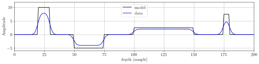
As we can see, the model presents some flat regions. Let's have a look to its first derivative:
D = o.FirstDerivative(x, stencil='forward')
Dx = D * x
fig, ax = plt.subplots()
ax.plot(x.plot(), 'k', label='model')
ax.stem(Dx.plot(), label='gradient', basefmt=':', use_line_collection=True)
ax.set_ylim(-12, 12)
ax.autoscale(enable=True, axis='x', tight=True)
plt.legend(loc="upper center")
ax.set_xlabel("Depth"), ax.set_ylabel("Amplitude")
plt.tight_layout(pad=.5)
plt.show()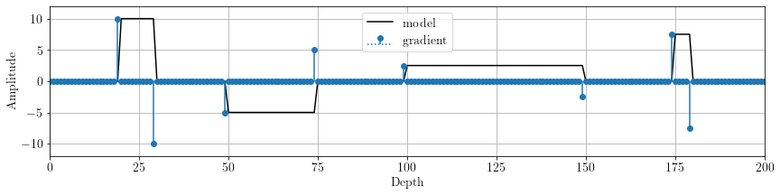
The model derivative is sparse! We can set up a SplitBregman solver:
problem = o.GeneralizedLasso(x.clone().zero(), d, G, reg=D, eps=.1)

SB = o.SplitBregman(o.BasicStopper(200), niter_inner=3, niter_solver=10,
                           linear_solver='LSQR', breg_weight=1., warm_start=True)
SB.setDefaults(save_obj=True, save_model=True)

SB.run(problem, verbose=False, inner_verbose=False)
its = "%d-%d-%d" % (len(SB.obj), SB.niter_inner, SB.niter_solver)
fig, ax = plt.subplots()
ax.plot(x.plot(), 'b', lw=2, label="true model")
ax.plot(problem.model.plot(), 'r', label="SB")
ax.legend(loc="upper center")
ax.set_ylim(-6, 12)
ax.autoscale(enable=True, axis='x', tight=True)
ax.set_xlabel(x.ax_info[0].l), ax.set_ylabel("Amplitude")
plt.suptitle(r'Split-Bregman %s, $\varepsilon=%.e$' % (its, problem.eps))
plt.show()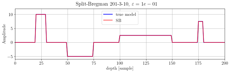
Let's check the convergence:
fig, ax = plt.subplots()
ax.semilogy(SB.obj / SB.obj[0], 'k', lw=2, label='Obj')
ax.semilogy(SB.obj_terms[:, 0] / SB.obj[0], 'b--', label=r"$0.5 \Vert \mathbf{Gx-d} \Vert_2^2$")
ax.semilogy(SB.obj_terms[:, 1] / SB.obj[0], 'r--', label=r"$\varepsilon \Vert \mathbf{Dx}\Vert_1$")
ax.set_ylim(1e-7, 1), ax.set_xlim(0, SB.stopper.niter)
ax.set_xlabel("Iterations"), ax.set_ylabel("Amplitude")
ax.legend(loc="right")

plt.suptitle(r'Split-Bregman %s, $\varepsilon=%.e$' % (its, problem.eps))
plt.show()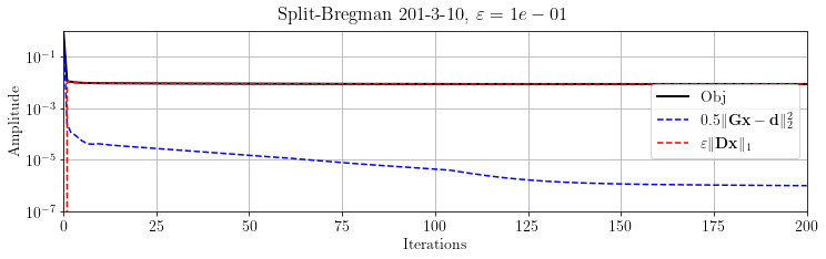
We can see that the L1 term reaches its final value after few iterations. Let's see the inverted model after 2 iterations:
fig, ax = plt.subplots()
ax.plot(x.plot(), 'b', lw=2, label="true model")
ax.plot(SB.model[2].plot(), 'r', label="SB")
ax.legend(loc="upper center")
ax.set_ylim(-6, 12)
ax.autoscale(enable=True, axis='x', tight=True)
ax.set_xlabel(x.ax_info[0].l), ax.set_ylabel("Amplitude")

plt.suptitle(r'Split-Bregman %s after 2, $\varepsilon=%.e$' % (its, problem.eps))
plt.show()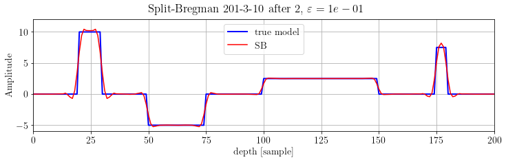
Just for comparison, let's solve the problem with CG and FISTA.
problemCG = o.LeastSquares(x.clone().zero(), d, G)
CG = o.CG(o.BasicStopper(1000))
CG.setDefaults(save_obj=True)
CG.run(problemCG, verbose=False)

fig, ax = plt.subplots()
ax.plot(x.plot(), 'b', lw=2, label="true model")
ax.plot(problemCG.model.plot(), 'r', label="CG")
ax.legend(loc="upper center")
ax.set_ylim(-6, 12)
ax.autoscale(enable=True, axis='x', tight=True)
ax.set_xlabel(x.ax_info[0].l), ax.set_ylabel("Amplitude")

plt.suptitle('Conjugate Gradient, %d it' % len(CG.obj))
plt.show()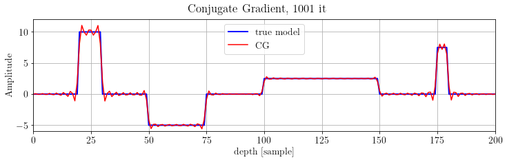
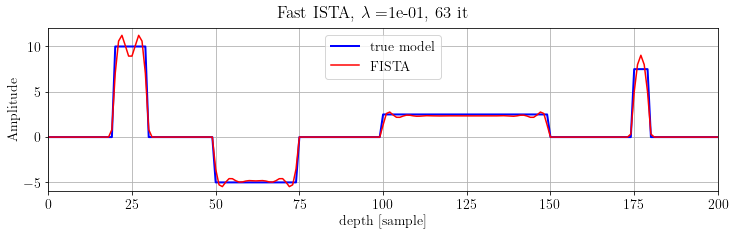
# compute maximum eigenvalue
maxeig = G.powerMethod()
print('FISTA α=%.6e' % (1/(maxeig**2)))
problemFISTA = o.Lasso(x.clone().zero(), d, G, lambda_value=.1, op_norm=maxeig**2)
FISTA = o.ISTA(o.BasicStopper(1000), fast=True)
FISTA.setDefaults(save_obj=True)
FISTA.run(problemFISTA, verbose=False)

fig, ax = plt.subplots(figsize=(12, 3))
ax.plot(x.plot(), 'b', lw=2, label="true model")
ax.plot(problemFISTA.model.plot(), 'r', label="FISTA")

ax.legend(loc="upper center")
ax.set_ylim(-6, 12)
ax.autoscale(enable=True, axis='x', tight=True)
ax.set_xlabel(x.ax_info[0].l), ax.set_ylabel("Amplitude")

plt.suptitle(r'Fast ISTA, $\lambda=$%.e, %d it' % (problemFISTA.lambda_value, len(FISTA.obj)))
plt.show()
FISTA α=1.570806e+00
Example 3: 2D Phantom Deconvolution
In this example we reconstruct a phantom CT image starting from a blurred acquisition. Again, we regularize the inversion by imposing the first derivative to be sparse
# model
x = o.VectorNumpy(np.load('./data/shepp_logan_phantom.npy').astype(np.float32)).scale(1 / 255.)

# operator
G = o.GaussianFilter(x, (3.,3.))

# data
d = G * x
fig, ax = plt.subplots(1, 2, figsize=(11,4))
ax[0].imshow(x.plot(), cmap='bone', clim=(0,1))
ax[0].grid(False)
ax[0].set_title('Model')
ax[1].imshow(d.plot(), cmap='bone', clim=(0,1))
ax[1].grid(False)
ax[1].set_title('Data')
plt.show()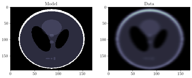
Problem and solver:
D = o.Gradient(x)
Dx = D * x

fig, ax = plt.subplots(1, 2, figsize=(11,4))
ax[0].imshow(Dx.vecs[1].plot(), cmap='bone')
ax[0].grid(False)
ax[0].set_title(r'$\nabla_h(x)$')
ax[1].imshow(Dx.vecs[0].plot(), cmap='bone')
ax[1].grid(False)
ax[1].set_title(r'$\nabla_v(x)$')
plt.show()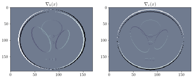
Just for comparison, let's solve the problem with CG.
problemCG = o.LeastSquares(x.clone().zero(), d, G)
CG = o.CG(o.BasicStopper(1000))
CG.setDefaults(save_obj=True)
CG.run(problemCG, verbose=False)
fig, ax = plt.subplots(1, 2, figsize=(11,4))
ax[0].imshow(x.plot(), cmap='bone', clim=(0,1))
ax[0].grid(False)
ax[0].set_title('Model')
ax[1].imshow(problemCG.model.plot(), cmap='bone', clim=(0,1))
ax[1].grid(False)
ax[1].set_title('Conjugate Gradient, %d it' % len(CG.obj))
plt.show()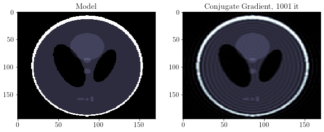
See the ringing effect there? Let's remove it by means of a regularizer!
problemSB = o.GeneralizedLasso(x.clone().zero(), d, G, reg=D, eps=1e-3)
SB = o.SplitBregman(o.BasicStopper(niter=200), niter_inner=3, niter_solver=10,
                           linear_solver='LSQR', breg_weight=1., warm_start=True)
SB.setDefaults(save_obj=True)
SB.run(problemSB, verbose=False, inner_verbose=False)
its = "%d-%d-%d" % (len(SB.obj), SB.niter_inner, SB.niter_solver)
fig, ax = plt.subplots(1, 2, figsize=(11,4))
ax[0].imshow(x.plot(), cmap='bone', clim=(0,1))
ax[0].grid(False)
ax[0].set_title('Model')
ax[1].imshow(problemSB.model.plot(), cmap='bone', clim=(0,1))
ax[1].grid(False)
ax[1].set_title(r'SB %s, $\varepsilon=%.e$' % (its, problemSB.eps))
plt.show()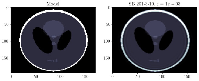
Again, let's evaluate the objective function terms
fig, ax = plt.subplots()
ax.semilogy(SB.obj / SB.obj[0], 'k', lw=2, label='Obj')
ax.semilogy(SB.obj_terms[:, 0] / SB.obj[0], 'b--', label=r"$0.5 \Vert \mathbf{Gx-d} \Vert_2^2$")
ax.semilogy(SB.obj_terms[:, 1] / SB.obj[0], 'r--', label=r"$\varepsilon \Vert \mathbf{Dx}\Vert_1$")
ax.set_ylim(1e-8, 1), ax.set_xlim(0, SB.stopper.niter)
ax.set_xlabel("Iterations")
ax.legend(loc="right")

plt.suptitle(r'Split-Bregman %s, $\varepsilon=%.e$' % (its, problem.eps))
plt.show()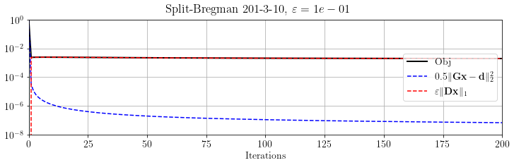
- Goldstein, T., & Osher, S. (2009). The Split Bregman Method for L1-Regularized Problems. SIAM Journal on Imaging Sciences, 2(2), 323–343. 10.1137/080725891
- Beck, A., & Teboulle, M. (2009). A Fast Iterative Shrinkage-Thresholding Algorithm for Linear Inverse Problems. SIAM Journal on Imaging Sciences, 2(1), 183–202. 10.1137/080716542