Least-Squares Reverse Time Migration through Devito and Automatic Differentiation¶

@Author: Francesco Picetti - picettifrancesco@gmail.com

In this tutorial, we put together torch's Automatic Differentiation abilities and the OccamyPy physical operators (well, actually Devito's) for RTM. Basically, we can write a standard pytorch optimization loop with the modeling provided by OccamyPy; the tricky part is to insert a linear operator (i.e., Born) in the AD graph.

To use this notebook, we need devito installed. On your occamypy-ready env, run

pip install --user git+https://github.com/devitocodes/devito.git

import torch
import occamypy as o
import born_devito as b

# Plotting
from matplotlib import rcParams
from mpl_toolkits.axes_grid1 import make_axes_locatable
import matplotlib.pyplot as plt
rcParams.update({
    'image.cmap'     : 'gray',
    'image.aspect'   : 'auto',
    'image.interpolation': None,
    'axes.grid'      : False,
    'figure.figsize' : (10, 6),
    'savefig.dpi'    : 300,
    'axes.labelsize' : 14,
    'axes.titlesize' : 16,
    'font.size'      : 14,
    'legend.fontsize': 14,
    'xtick.labelsize': 14,
    'ytick.labelsize': 14,
    'text.usetex'    : True,
    'font.family'    : 'serif',
    'font.serif'     : 'Latin Modern Roman',
})

WARNING! DATAPATH not found. The folder /tmp will be used to write binary files

/nas/home/fpicetti/miniconda3/envs/occd/lib/python3.10/site-packages/dask_jobqueue/core.py:20: FutureWarning: tmpfile is deprecated and will be removed in a future release. Please use dask.utils.tmpfile instead.
  from distributed.utils import tmpfile

Setup¶

args = dict(
    filter_sigma=(1, 1),
    spacing=(10., 10.),  # meters
    shape=(101, 101),    # samples
    nbl=20,              # samples
    nreceivers=51,
    src_x=[500],         # meters
    src_depth=20.,       # meters
    rec_depth=30.,       # meters
    t0=0.,
    tn=2000.,            # Simulation lasts 2 second (in ms)
    f0=0.010,            # Source peak frequency is 10Hz (in kHz)
    space_order=5,
    kernel="OT2",
    src_type='Ricker',
)

def unpad(model, nbl: int = args["nbl"]):
    return model[nbl:-nbl, nbl:-nbl]

create hard model and migration model

model_true, model_smooth, water = b.create_models(args)
model = o.VectorNumpy(model_smooth.vp.data.__array__())
model.ax_info = [
    o.AxInfo(model_smooth.vp.shape[0], model_smooth.origin[0] - model_smooth.nbl * model_smooth.spacing[0],
             model_smooth.spacing[0], "x [m]"),
    o.AxInfo(model_smooth.vp.shape[1], model_smooth.origin[1] - model_smooth.nbl * model_smooth.spacing[1],
             model_smooth.spacing[1], "z [m]")]
model_extent = [0., 1000., 1000., 0.]

Define acquisition geometry

rec = b.build_rec_coordinates(model_true, args)
src = [b.build_src_coordinates(x, args["src_depth"]) for x in args["src_x"]]

create the common shot gather (CSG) data¶

d = o.VectorTorch(b.propagate_shots(model=model_true, src_pos=src, rec_pos=rec, param=args))
assert d[:].requires_grad is False

fig, axs = plt.subplots(1, 1, sharey=True)
axs.imshow(d.plot(), clim=o.plot.clim(d[:]),
           extent=[d.ax_info[1].o, d.ax_info[1].last, d.ax_info[0].last, d.ax_info[0].o])
axs.set_xlabel(d.ax_info[1].l)
axs.set_ylabel(d.ax_info[0].l)
fig.suptitle(r"Nonlinear data: $\mathbf{d}$")
plt.tight_layout()
plt.show()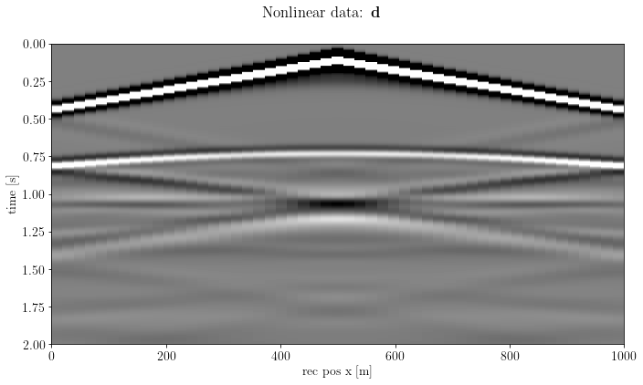

Instantiate the Born operator...¶

B = b.BornSingleSource(velocity=model_smooth, src_pos=src[0], rec_pos=rec, args=args)

... and cast it to an Autograd function¶

B_ = o.torch.AutogradFunction(B)

Learning paradigm¶

instantiate the model as a "learnable" vector, i.e., a new kind of VectorTorch that encapsulate a tensor attached to the AD graph

m = o.torch.VectorAD(torch.zeros(model.shape), ax_info=model.ax_info)

m.setDevice(None)

assert m[:].requires_grad is True

instantiate the optimizer that will work on the model

opt = torch.optim.SGD([m.getNdArray()], lr=1)

define the objective function terms: the mean squared error...

mse = torch.nn.MSELoss().to(m.device)

and more complex terms (the TV, for example) that can be based on OccamyPy operators!

G = o.torch.AutogradFunction(o.FirstDerivative(model, axis=0))
l1 = torch.nn.L1Loss().to(m.device)
tv = lambda x: l1(G(x), torch.zeros_like(x))

Optimization loop¶

epochs = 10

for epoch in range(epochs):
    
    # modeling
    d_ = B_(m)
    
    # note: things can be a lot complicated! Deep Priors, CNN-based denoisers, ecc ecc
    
    # objective function
    loss = mse(d_.float(), d[:]) + 0.1 * tv(m.getNdArray())
    
    # model update
    opt.zero_grad()
    loss.backward()
    opt.step()
    
    # log
    print("Epoch %s, obj = %.2e" % (str(epoch).zfill(3), loss))

Epoch 000, obj = 1.44e+00
Epoch 001, obj = 1.02e+00
Epoch 002, obj = 8.32e-01
Epoch 003, obj = 7.27e-01
Epoch 004, obj = 6.63e-01
Epoch 005, obj = 6.20e-01
Epoch 006, obj = 5.89e-01
Epoch 007, obj = 5.66e-01
Epoch 008, obj = 5.47e-01
Epoch 009, obj = 5.32e-01

fig, axs = plt.subplots(1, 1, sharey=True)
axs.imshow(unpad(m.plot()).T, clim=o.plot.clim(m.plot()), extent=model_extent)
axs.set_xlabel(m.ax_info[0].l)
axs.set_ylabel(m.ax_info[1].l)
fig.suptitle(r"$\hat{\mathbf{m}} = \arg \min \Vert \mathbf{B}\mathbf{m} - \mathbf{d} \Vert_2^2 \quad$" + f"after {epochs} iterations of SGD with lr={opt.param_groups[0]['lr']}")
plt.tight_layout()
plt.show()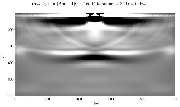

Shot-wise Dask distribution: WIP¶

In principle, an AutogradFunction can be casted also for Dask-distributed operators. However, distributing a shot to each workers (as done in the previous tutorial) will require the objective function to be computed on different workers, too.

Therefore, we need to merge the distribution paradigms of Dask and PyTorch. Any help will be appreciated!

Notebooks

Traveltime tomography for Seismic Exploration