Traveltime tomography using the Eikonal equation (2D case)
@Author: Ettore Biondi - ebiondi@caltech.edu
To use this notebook, we need pykonal installed. In your env, you can install it by:
conda install cythonpip install git+https://github.com/malcolmw/pykonal@0.2.3b3
import numpy as np
import occamypy as o
import eikonal2d as k

# Plotting
from matplotlib import rcParams
from mpl_toolkits.axes_grid1 import make_axes_locatable
import matplotlib.pyplot as plt
rcParams.update({
    'image.cmap'     : 'jet',
    'image.aspect'   : 'equal',
    'axes.grid'      : True,
    'figure.figsize' : (19, 8),
    'savefig.dpi'    : 300,
    'axes.labelsize' : 14,
    'axes.titlesize' : 16,
    'font.size'      : 14,
    'legend.fontsize': 14,
    'xtick.labelsize': 14,
    'ytick.labelsize': 14,
})
WARNING! DATAPATH not found. The folder /tmp will be used to write binary files
/Library/Frameworks/Python.framework/Versions/3.9/lib/python3.9/site-packages/dask_jobqueue/core.py:20: FutureWarning: tmpfile is deprecated and will be removed in a future release. Please use dask.utils.tmpfile instead.
  from distributed.utils import tmpfile
# Fast-Marching-Method (FMM)
dx = dz = 0.1
nx, nz = 201, 101
x = np.linspace(0,(nx-1)*dx, nx)
z = np.linspace(0,(nz-1)*dz, nz)

# Velocity model
vv = o.VectorNumpy((nx,nz), ax_info=[o.AxInfo(nx, 0, dx, "x [km]"), o.AxInfo(nz, 0, dz, "z [km]")])
vv[:] = 1. + 0.1*z
# Source/Receiver positions
SouPos = np.array([[0,nz-1], [int(nx/2), nz-1], [nx-1, nz-1]])
RecPos = np.array([[ix,0] for ix in np.arange(0,nx)])
# Data vector
tt_data = o.VectorNumpy((SouPos.shape[0], RecPos.shape[0]),
ax_info=[o.AxInfo(SouPos.shape[0], 0, 1, "rec_id"), vv.ax_info[0]])
tt_data.zero()
# Setting Forward non-linear operator
Eik2D_Op = k.EikonalTT_2D(vv, tt_data, SouPos, RecPos)
Eik2D_Op.forward(False, vv, tt_data)# Plotting traveltime vector
fig, ax = plt.subplots()
ax.plot(tt_data.ax_info[1].plot(), tt_data[0], lw=2)
ax.plot(tt_data.ax_info[1].plot(), tt_data[1], lw=2)
ax.plot(tt_data.ax_info[1].plot(), tt_data[2], lw=2)
ax.grid()
plt.xlabel(tt_data.ax_info[1].l)
plt.ylabel("Traveltime [s]")
ax.set_ylim(0, 25)
ax.set_xlim(tt_data.ax_info[1].o, tt_data.ax_info[1].last)
plt.tight_layout()
plt.show()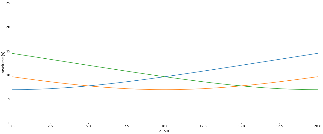
# Dot-product test for the linearized Eikonal equation in 1D
Eik2D_Lin_Op = k.EikonalTT_lin_2D(vv, tt_data, SouPos, RecPos)
Eik2D_Lin_Op.dotTest(True)
Dot-product tests of forward and adjoint operators
--------------------------------------------------
Applying forward operator add=False
Runs in: 2.6184580326080322 seconds
Applying adjoint operator add=False
Runs in: 3.965895175933838 seconds
Dot products add=False: domain=1.542013e+00 range=1.542013e+00
Absolute error: 8.881784e-16
Relative error: 5.759863e-16
Applying forward operator add=True
Runs in: 0.11392402648925781 seconds
Applying adjoint operator add=True
Runs in: 0.514909029006958 seconds
Dot products add=True: domain=3.084026e+00 range=3.084026e+00
Absolute error: 8.881784e-16
Relative error: 2.879932e-16
-------------------------------------------------
Inversion
# Fast-Marching-Method (FMM)
# dx = dz = 0.05
dx = dz = 0.1
nx, nz = 201, 101
x = np.linspace(0,(nx-1)*dx, nx)
z = np.linspace(0,(nz-1)*dz, nz)
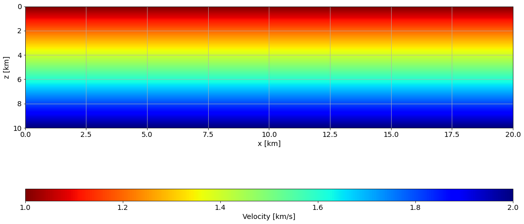
# Background Velocity model
vv0 = o.VectorNumpy((nx,nz), ax_info=[o.AxInfo(nx, 0, dx, "x [km]"), o.AxInfo(nz, 0, dz, "z [km]")])
vv0[:] = 1.0 + z*0.1
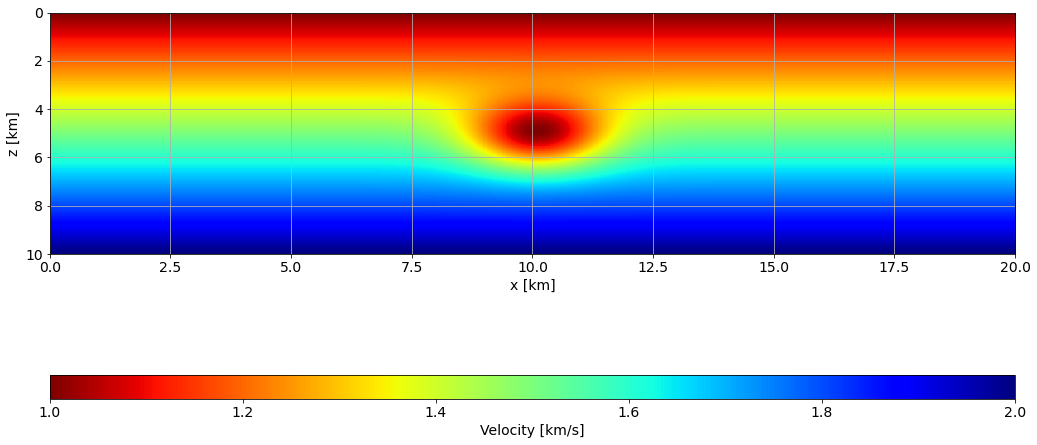
# Gaussian anomaly
zz, xx = np.meshgrid(z, x)
dst = np.sqrt(xx*xx+zz*zz)
sigma = 1.0
xloc = 101*dx
zloc = 51*dz
gauss = np.exp(-( ((xx-xloc)**2 + (zz-zloc)**2) / (2.0*sigma**2)))
# Constructing true model
vv = vv0.clone()
vv[:] -= gauss*0.5fig, ax = plt.subplots()
im = ax.imshow(vv0.plot().T, extent=[x[0], x[-1], z[-1], z[0]], aspect=0.5, cmap="jet_r")
ax = plt.gca()
plt.xlabel(vv0.ax_info[0].l)
plt.ylabel(vv0.ax_info[1].l)
cbar = plt.colorbar(im, orientation="horizontal",
cax=make_axes_locatable(ax).append_axes("bottom", size="5%", pad=0))
cbar.set_label('Velocity [km/s]')
plt.tight_layout()
plt.show()
ax.grid()/var/folders/q3/lmm60bhj01xcxkxyn8zc_mdm0000gn/T/ipykernel_99151/375083392.py:6: MatplotlibDeprecationWarning: Auto-removal of grids by pcolor() and pcolormesh() is deprecated since 3.5 and will be removed two minor releases later; please call grid(False) first.
cbar = plt.colorbar(im, orientation="horizontal",
fig, ax = plt.subplots()
im = ax.imshow(vv.plot().T, extent=[x[0], x[-1], z[-1], z[0]], aspect=0.5, cmap="jet_r")
ax = plt.gca()
plt.xlabel(vv0.ax_info[0].l)
plt.ylabel(vv0.ax_info[1].l)
cbar = plt.colorbar(im, orientation="horizontal",
                    cax=make_axes_locatable(ax).append_axes("bottom", size="5%", pad=0))
cbar.set_label('Velocity [km/s]')
plt.tight_layout()
plt.show()
ax.grid()
/var/folders/q3/lmm60bhj01xcxkxyn8zc_mdm0000gn/T/ipykernel_99151/4118034870.py:6: MatplotlibDeprecationWarning: Auto-removal of grids by pcolor() and pcolormesh() is deprecated since 3.5 and will be removed two minor releases later; please call grid(False) first.
cbar = plt.colorbar(im, orientation="horizontal",
# Source/Receiver positions
SouPos = np.array([[ix,nz-1] for ix in np.arange(0,nx,20)])
RecPos = np.array([[ix,0] for ix in np.arange(0,nx)])

# Data vector
tt_data = o.VectorNumpy((SouPos.shape[0], RecPos.shape[0]),
                        ax_info=[o.AxInfo(SouPos.shape[0], 0, 1, "rec_id"), vv.ax_info[0]])

# Instantiating non-linear operator
Eik2D_Op = k.EikonalTT_2D(vv, tt_data, SouPos, RecPos)
Eik2D_Lin_Op = k.EikonalTT_lin_2D(vv, tt_data, SouPos, RecPos, tt_maps=Eik2D_Op.tt_maps)
Eik2D_NlOp = o.NonlinearOperator(Eik2D_Op, Eik2D_Lin_Op, Eik2D_Lin_Op.set_vel)
# Creating observed data
Eik2D_Op.forward(False, vv, tt_data)
tt_data_obs = tt_data.clone()# Plotting traveltime vector
fig, ax = plt.subplots(figsize=(10,5))
for ids in range(SouPos.shape[0]):
ax.plot(tt_data.ax_info[1].plot(), tt_data[ids], lw=2)
ax.grid()
plt.xlabel(tt_data.ax_info[1].l)
plt.ylabel("Traveltime [s]")
ax.set_ylim(5.0, 15.0)
ax.set_xlim(tt_data.ax_info[1].o, tt_data.ax_info[1].last)
ax.invert_yaxis()
plt.tight_layout()
plt.show()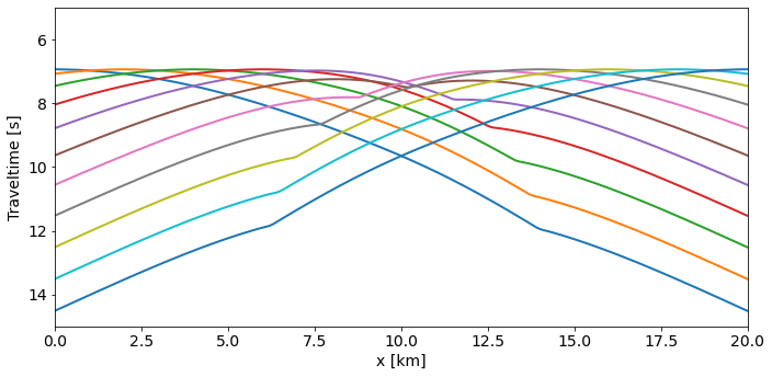
# instantiate solver
BFGSBsolver = o.LBFGS(o.BasicStopper(niter=25, tolg_proj=1e-32), m_steps=30)

# Creating problem object using Smoothing filter
G = o.GaussianFilter(vv0, 1.5)

Eik2D_Inv_NlOp = o.NonlinearOperator(Eik2D_Op, Eik2D_Lin_Op * G, Eik2D_Lin_Op.set_vel)

L2_tt_prob = o.NonlinearLeastSquares(vv0.clone(), tt_data_obs, Eik2D_Inv_NlOp,
                                     minBound=vv0.clone().set(1.),  # min velocity: 1 km/s
                                     maxBound=vv0.clone().set(2.5)) # max velocity: 2.5 km/s
BFGSBsolver.run(L2_tt_prob, verbose=True)##########################################################################################
Limited-memory Broyden-Fletcher-Goldfarb-Shanno (L-BFGS) algorithm
Maximum number of steps to be used for Hessian inverse estimation: 30
Restart folder: /tmp/restart_2022-04-26T08-05-57.869068/
##########################################################################################
iter = 00, obj = 2.48052e+01, resnorm = 7.04e+00, gradnorm = 8.73e+00, feval = 1, geval = 1
iter = 01, obj = 8.19519e+00, resnorm = 4.05e+00, gradnorm = 5.07e+00, feval = 2, geval = 2
iter = 02, obj = 2.58445e+00, resnorm = 2.27e+00, gradnorm = 1.52e+00, feval = 3, geval = 3
iter = 03, obj = 1.23840e+00, resnorm = 1.57e+00, gradnorm = 9.19e-01, feval = 4, geval = 4
iter = 04, obj = 3.15355e-01, resnorm = 7.94e-01, gradnorm = 4.07e-01, feval = 5, geval = 5
iter = 05, obj = 2.03645e-01, resnorm = 6.38e-01, gradnorm = 2.46e-01, feval = 6, geval = 6
iter = 06, obj = 9.79590e-02, resnorm = 4.43e-01, gradnorm = 1.75e-01, feval = 7, geval = 7
iter = 07, obj = 4.01127e-02, resnorm = 2.83e-01, gradnorm = 1.04e-01, feval = 8, geval = 8
iter = 08, obj = 2.53056e-02, resnorm = 2.25e-01, gradnorm = 7.52e-02, feval = 9, geval = 9
iter = 09, obj = 1.84552e-02, resnorm = 1.92e-01, gradnorm = 5.70e-02, feval = 10, geval = 10
iter = 10, obj = 1.35375e-02, resnorm = 1.65e-01, gradnorm = 3.87e-02, feval = 11, geval = 11
iter = 11, obj = 1.13803e-02, resnorm = 1.51e-01, gradnorm = 3.05e-02, feval = 12, geval = 12
iter = 12, obj = 9.72617e-03, resnorm = 1.39e-01, gradnorm = 2.81e-02, feval = 13, geval = 13
iter = 13, obj = 7.87789e-03, resnorm = 1.26e-01, gradnorm = 2.74e-02, feval = 14, geval = 14
iter = 14, obj = 5.84876e-03, resnorm = 1.08e-01, gradnorm = 2.24e-02, feval = 15, geval = 15
iter = 15, obj = 4.64104e-03, resnorm = 9.63e-02, gradnorm = 1.48e-02, feval = 16, geval = 16
iter = 16, obj = 4.15353e-03, resnorm = 9.11e-02, gradnorm = 1.24e-02, feval = 17, geval = 17
iter = 17, obj = 3.77232e-03, resnorm = 8.69e-02, gradnorm = 1.23e-02, feval = 18, geval = 18
iter = 18, obj = 3.22827e-03, resnorm = 8.04e-02, gradnorm = 1.25e-02, feval = 19, geval = 19
iter = 19, obj = 2.76429e-03, resnorm = 7.44e-02, gradnorm = 1.17e-02, feval = 20, geval = 20
iter = 20, obj = 2.43497e-03, resnorm = 6.98e-02, gradnorm = 1.11e-02, feval = 21, geval = 21
iter = 21, obj = 2.16737e-03, resnorm = 6.58e-02, gradnorm = 1.12e-02, feval = 22, geval = 22
iter = 22, obj = 1.89961e-03, resnorm = 6.16e-02, gradnorm = 1.12e-02, feval = 23, geval = 23
iter = 23, obj = 1.66281e-03, resnorm = 5.77e-02, gradnorm = 9.80e-03, feval = 24, geval = 24
iter = 24, obj = 1.49744e-03, resnorm = 5.47e-02, gradnorm = 8.04e-03, feval = 25, geval = 25
iter = 25, obj = 1.38691e-03, resnorm = 5.27e-02, gradnorm = 7.12e-03, feval = 26, geval = 26
Terminate: maximum number of iterations reached
##########################################################################################
Limited-memory Broyden-Fletcher-Goldfarb-Shanno (L-BFGS) algorithm end
##########################################################################################
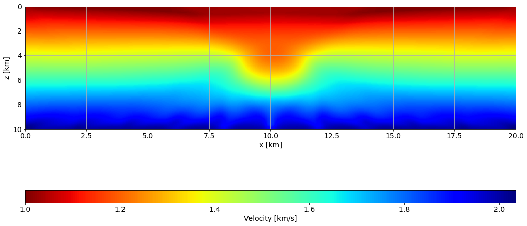
fig, ax = plt.subplots()
im = ax.imshow(L2_tt_prob.model.plot().T, extent=[x[0], x[-1], z[-1], z[0]], aspect=0.5, cmap="jet_r")
ax = plt.gca()
plt.xlabel(vv0.ax_info[0].l)
plt.ylabel(vv0.ax_info[1].l)
cbar = plt.colorbar(im, orientation="horizontal",
                    cax=make_axes_locatable(ax).append_axes("bottom", size="5%", pad=0))
cbar.set_label('Velocity [km/s]')
plt.tight_layout()
plt.show()
ax.grid()
/var/folders/q3/lmm60bhj01xcxkxyn8zc_mdm0000gn/T/ipykernel_99151/2870563539.py:6: MatplotlibDeprecationWarning: Auto-removal of grids by pcolor() and pcolormesh() is deprecated since 3.5 and will be removed two minor releases later; please call grid(False) first.
cbar = plt.colorbar(im, orientation="horizontal",