Basic Normalizing Flow Training and Sampling
This notebook is the first in a series of InvertibleNetworks.jl. In this tutorial, we will layout the basic theory behind Normalizing Flows (NFs) and how to use the implementations in InvertibleNetworks.jl to train and sample from a basic NF. The following notebook in the series demonstrates how to train a conditional normalizing flow. You can also learn the concept and ideology of InvertibleNetworks.jl package in the JuliaCon 2021 presentation with the youtube video here.
In this tutorial, we train an NF using the GLOW architecture, which implements:
- Affine couplying layer from Real-NVP
- Ability to activate multiscale for efficient training and compressive behavior in latent
- ActNorms for stable training
- 1x1 Convolutions for channel mixing between affine couplying layers
using InvertibleNetworks
using LinearAlgebra
using PyPlot
using Flux
using Random

import Flux.Optimise: ADAM, update!
Random.seed!(1234)

PyPlot.rc("font", family="serif");
What is normalizing flow
Normalizing flow (NF) is a type of invertible neural network (INN) containing a series of invertible layers, which aims to learn a probability distribution (e.g. cat images). After training, NF can output a white noise image given an input as a cat image in the distribution. Thanks to its invertibility, we can easily draw sample images from the "cat" distribution by drawing random white noise and apply the inverse of the NF.
Target distribution
For this example, we will learn to sample from the 2-D Rosenbrock distribution. Accessible in InvertibleNetworks.jl using its colloquial name: the "banana" distribution. The idea of invertible networks is that we want to learn an invertible nonlinear mapping such that
where is the network parameter, samples from the target distribution, samples from Gaussian distribution (white noise). After training, NF can sample from the target distribution via evaluating the inverse of NF on white noise, i.e., . Let's first generate a training set and plot the target banana distribution.
n_train = 60000;
X_train = sample_banana(n_train);
size(X_train) #(nx, ny, n_channels, n_samples) Note: we put 2 dimensions as channels
(1, 1, 2, 60000)fig = figure(); title(L"x \sim p_x(x)")
scatter(X_train[1,1,1,1:400], X_train[1,1,2,1:400]; alpha=0.4, label = L"x \sim p_{X}(x)");
xlabel(L"x_1"); ylabel(L"x_2");
xlim(-4,4); ylim(0,30);
legend();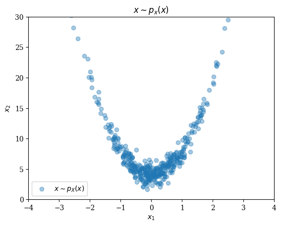
Change of variables formula
This formula allows us to evaluate the density of a sample under a monotone function .
This density estimation is what gives us a maximum likelihood framework for training our parameterized Normalizing Flow .
Training a normalizing flow
NF training is based on likelihood maximization of the parameterized model under the log likelihood of samples from the data distribution X:
We approximate the expectation with Monte Carlo samples from the training dataset:
We make this a minimization problem by looking at the negative loglikelihood and then the change of variabes formula makes this:
This means that you apply your network to your data and want to look like Normal noise. The log det of the jacobian term is making sure that we learn a distribution.
Calling G.backward will set all the gradients of the trainable parameters in G. We can access these parameters and their gradients with get_params and update them with the optimizer of our choice.
Note: since the network is invertible, we do not need to save intermediate states to calculate the gradient. Instead, we only provide the G.backward function with the final output Z and it will recalculate the intermediate states to calculate the gradients at each layer while backpropagating the residual dZ.
function loss(G, X)
    batch_size = size(X)[end]

    Z, lgdet = G.forward(X)

    l2_loss = 0.5*norm(Z)^2 / batch_size  #likelihood under Normal Gaussian training
    dZ = Z / batch_size                   #gradient under Normal Gaussian training

    G.backward(dZ, Z)  #sets gradients of G wrt output and also logdet terms

    return (l2_loss, lgdet)
end
loss (generic function with 1 method)nx = 1
ny = 1
#network architecture
n_in = 2 #put 2d variables into 2 channels
n_hidden = 16
levels_L = 1
flowsteps_K = 10
G = NetworkGlow(n_in, n_hidden, levels_L, flowsteps_K;)
#G = G |> gpu
#training parameters
batch_size = 150
maxiter = cld(n_train, batch_size)
lr = 9f-4
opt = ADAM(lr)
loss_l2_list = zeros(maxiter)
loss_lgdet_list = zeros(maxiter)
for j = 1:maxiter
Base.flush(Base.stdout)
idx = ((j-1)*batch_size+1):(j*batch_size)
X = X_train[:,:,:,idx]
#x = x |> gpu
losses = loss(G, X) #sets gradients of G
loss_l2_list[j] = losses[1]
loss_lgdet_list[j] = losses[2]
(j%50==0) && println("Iteration=", j, "/", maxiter,
"; f l2 = ", loss_l2_list[j],
"; f lgdet = ",loss_lgdet_list[j],
"; f nll objective = ",loss_l2_list[j] - loss_lgdet_list[j])
for p in get_params(G)
update!(opt,p.data,p.grad)
end
endIteration=50/400; f l2 = 0.9015696207682292; f lgdet = -1.4711344242095947; f nll objective = 2.372704044977824
Iteration=100/400; f l2 = 1.1610940551757813; f lgdet = -0.8267961740493774; f nll objective = 1.9878902292251588
Iteration=150/400; f l2 = 1.0150911458333334; f lgdet = -0.5953445434570312; f nll objective = 1.6104356892903646
Iteration=200/400; f l2 = 0.9457177734375; f lgdet = -0.43935251235961914; f nll objective = 1.385070285797119
Iteration=250/400; f l2 = 0.9822599283854166; f lgdet = -0.22864198684692383; f nll objective = 1.2109019152323404
Iteration=300/400; f l2 = 1.040484415690104; f lgdet = -0.24717164039611816; f nll objective = 1.2876560560862222
Iteration=350/400; f l2 = 0.9652345784505209; f lgdet = -0.23387017846107483; f nll objective = 1.1991047569115958
Iteration=400/400; f l2 = 0.8642562866210938; f lgdet = -0.07342183589935303; f nll objective = 0.9376781225204468
Check training objective log
There are various ways to train a NF:
- train your network to convergence of objective
- use earlystopping to prevent overfitting
- check normality of with qq plots
- as a heuristic simply observe until it looks normal under the eyeball norm.
gt_l2 = 0.5*nx*ny*n_in #likelihood of gaussian noise

fig, axs = subplots(3, 1, sharex=true)
fig.subplots_adjust(hspace=0)

axs[1].plot(loss_l2_list, color="black", linewidth=0.6);
axs[1].axhline(y=gt_l2,color="red",linestyle="--",label="Normal Noise Likelihood")
axs[1].set_ylabel("L2 Norm")
axs[1].yaxis.set_label_coords(-0.09, 0.5)
axs[1].legend()

axs[2].plot(loss_lgdet_list, color="black", linewidth=0.6);
axs[2].set_ylabel("Log DET")
axs[2].yaxis.set_label_coords(-0.09, 0.5)

axs[3].plot(loss_l2_list - loss_lgdet_list, color="black", linewidth=0.6);
axs[3].set_ylabel("Full Objective")
axs[3].yaxis.set_label_coords(-0.09, 0.5)
axs[3].set_xlabel("Parameter Update") 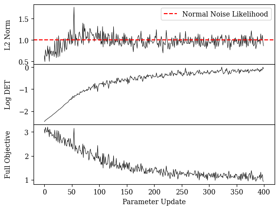
PyObject Text(0.5, 24.0, 'Parameter Update')Testing a Normalizing Flow
Since we have access to in the simple 2D Rosenbrock distribution, we can verify that generative samples from our trained network look like they come from .
We can verify this visually (easy since this is a 2D dataset) and under the ground truth density of .
Let's start by taking samples from
num_test_samples = 500;
Z_test = randn(Float32,nx,ny,n_in, num_test_samples);

fig = figure(); title(L"z \sim p_{Z}(z)")
ax = fig.add_subplot(111);
scatter(Z_test[1,1,1,:], Z_test[1,1,2,:]; alpha=0.4, color="black", label = L"z \sim p_{Z}(z)");
xlabel(L"z_1"); ylabel(L"z_2");
xlim(-5,5); ylim(-5,5);
legend();
ax.set_aspect(1);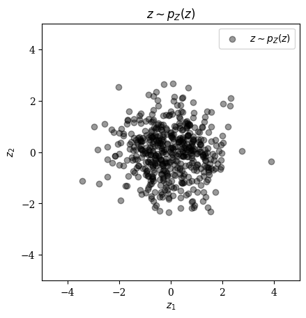
Pass Normal samples through the inverse network
X_test = G.inverse(Z_test);trans_num = 150
start_points = [(Z_test[1,1,1,i], Z_test[1,1,2,i]) for i in 1:trans_num]
end_points = [(X_test[1,1,1,i], X_test[1,1,2,i]) for i in 1:trans_num]
fig = figure(figsize=(7,9)); title(L"Transformed latent $z \rightarrow x=G^{-1}_\theta(z)$");
ax = fig.add_subplot(111)
for line in zip(start_points, end_points)
plot([line[1][1],line[2][1]], [line[1][2] ,line[2][2]], alpha=0.2, linewidth=0.3, color="black")
scatter(line[1][1], line[1][2], marker="o",alpha=0.4, color="black")
scatter(line[2][1], line[2][2], marker="o",alpha=0.4, color="orange")
end
xlabel("First Dimension"); ylabel("Second Dimension");
ylim(-2.5,20); xlim(-2.5,2.5); ax.set_aspect(1)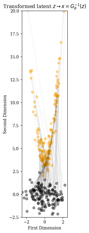
Visually compare generative samples with samples from the ground truth density
fig = figure(); title(L"Generative samples of  $x \sim p_{\theta}(x)$")
scatter(X_train[1,1,1,1:400], X_train[1,1,2,1:400]; alpha=0.4, label = L"x \sim p_{X}(x)");
scatter(X_test[1,1,1,1:400], X_test[1,1,2,1:400]; alpha=0.4, color="orange", label = L"x \sim p_{\theta}(x) = G_\theta^{-1}(z)");
xlabel(L"x_1"); ylabel(L"x_2");
xlim(-4,4); ylim(0,30);
legend();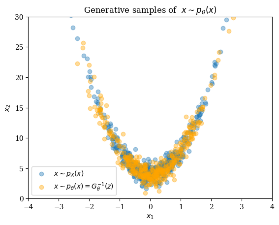
Below are a list of publications in SLIM group that use InvertibleNetworks.jl for seismic/medical imaging, and in general, inverse problems: