Introduction to JOLI
JOLI.jl is a Julia framework for constructing matrix-free linear operators with explicit domain/range type control and applying them in basic algebraic matrix-vector operations. This notebook mainly covers 3 things:
How to build a linear operator in JOLI, and verify its correctness.
How to solve a linear inverse problem where is a linear operator defined by JOLI.
How JOLI interacts with machine learning toolbox Flux.jl and optimization toolbox Optim.jl via ChainRules.jl.
Build a linear operator
We start by loading a few packages.
using LinearAlgebra, FFTW, JOLI, PyPlot, Random, IterativeSolvers, GenSPGL, Test;
using Optim, Flux;
Random.seed!(4321);
The JOLI toolbox gives a way to represent matrices implicitly. Instead of storing all entries in a matrix, JOLI only needs to store the forward and adjoint actions of this matrix on a vector, and the metadata (domain/range types etc). This is quite important when working with large-scale linear systems, where the linear operator can only be stored in a matrix-free way to fit into memory.
For example, we can construct a convolution operator given its kernel via JOLI toolbox. We first set up the convolution kernel as below
t = 0:.001:2';   # time interval
N = length(t);   # length
w = (1 .-2*1e3*(t .-.2).^2).*exp.(-1e3*(t .-.2).^2);    # convolution kernel
figure();plot(t, w);title("convolution kernel w");xlabel("time [s]");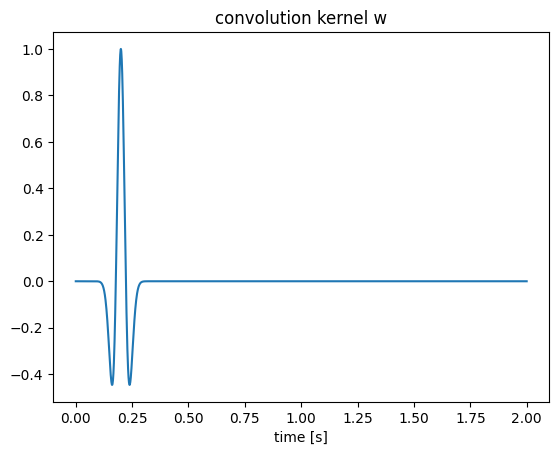
We know that convolution can be computed easily thanks to Fourier transform---i.e.,
where denotes the Fourier transform, denotes convolution, and denotes element-wise multiplication. Therefore, we can use the pre-defined linear operators in JOLI (joDFT for Fourier transform and joDiag for diagonal matrix) to construct the convolution operator A as
F = joDFT(N; DDT=Float64, RDT=ComplexF64);
W = joDiag(fft(w); DDT=ComplexF64, RDT=ComplexF64);
A = F' * W * F;
In general, JOLI provides a variety of linear operators that are frequently used in the scientific computing community, such as restriction operators, compressive sensing matrices, Fourier/wavelet/curvelet transforms, to name only a few. If you want to use common linear operators, we suggest you first check the JOLI reference guide to find pre-existing ones. In case you want to define something exotic enough that doesn’t exist yet in the JOLI package, you can still construct your own JOLI operator by providing the forward and adjoint actions of the operator. The code block below is a dummy example to demonstrate how to build a linear operator of dense matrix (although there is already joMatrix to do this):
M = randn(N, N)                   # a dense matrix
M1 = joLinearFunctionFwd_A(N, N,  # input and output size
        x -> M * x,                             # forward evaluation
        x -> adjoint(M) * x,                    # adjoint evaluation
        Float64, Float64; name="DIYOp");        # domain and range types, operator name
We can access the types of domain/range and size of M1 via native julia functions
println("size(M1) is ", size(M1))
println("domain type is ", deltype(M1))
println("range type is ", reltype(M1))
size(M1) is (2001, 2001)
domain type is Float64
range type is Float64
After we define the linear operator M1, we should verify its correctness by linearity test and adjoint test
a1 = randn(Float64, N);
a2 = randn(Float64, N);
@test isapprox(M1 * a1 + M1 * a2, M1 * (a1 + a2));        # linearity test
@test isapprox(dot(a1, M1 * a2), dot(M1' * a1, a2));      # adjoint(dot) test
JOLI also provides these testing functions so that it generates the testing vectors and runs the test for you
@test islinear(M1)[1];
@test isadjoint(M1)[1];
In case you've built your own JOLI operator and you find this operator is generally applicable to a broader community, we highly encourage and appreciate your contribution via a pull request to add your DIY operator in JOLI.
Solve with the built linear operator
Now we have successfully defined a convolution operator A with JOLI toolbox. We can then solve a linear inverse problem
using iterative solvers. In this tutorial, we set up a ground truth x as a sparse vector, and use 2 iterative methods to solve for x---LSQR and spgl1. Notice that these iterative methods only require the forward and adjoint evaluations of A, which are both provided by our JOLI operator. Thanks to the power of abstraction in Julia, we do not need to overload these iterative algorithms. These julia native algorithms work out of the box.
# set up the ground truth x
k = 20;                   # number of sparse entries
x = zeros(N);
x[rand(1:N, k)] = randn(k);
figure();plot(t, x);title("ground truth x");xlabel("time [s]");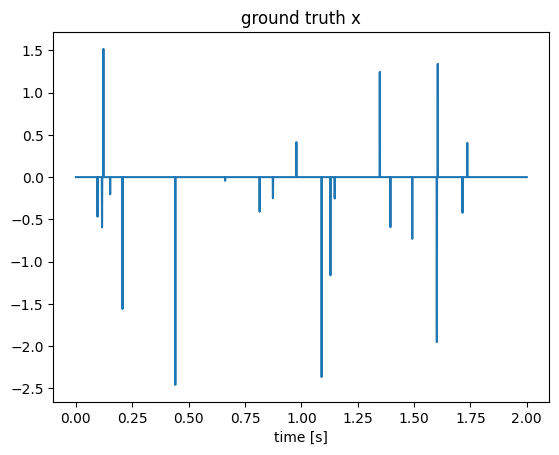
We then generate a noisy measurement b via perturbing the forward evaluation by a noise term e.
e = 1e-3 * randn(N);    # noise
b = A * x + e;          # noisy measurement
Then we can first solve for x using LSQR in IterativeSolvers.jl package, defined here.
x1 = lsqr(A, b; maxiter=500);
figure();plot(t, x1);title("solution from LSQR");xlabel("time [s]");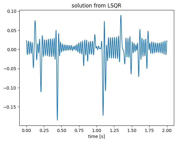
We can see the recovery is somehow noisy because the convolution operator has a null space and LSQR searches for a minimal 2-norm solution. Since the ground truth signal is sparse, we can use spgl1 algorithm to solve for x, which pursues a sparse solution. We adopt the spgl1 algorithm implemented in GenSPGL.jl package, defined here.
x2, _, _, _ = spgl1(A, b, options = spgOptions(iterations=500, verbosity=0));
figure();plot(t, x2);title("solution from spgl1");xlabel("time [s]");
WARNING: options.stepMin is below the precision of the data type. Setting to 10*eps(DT)
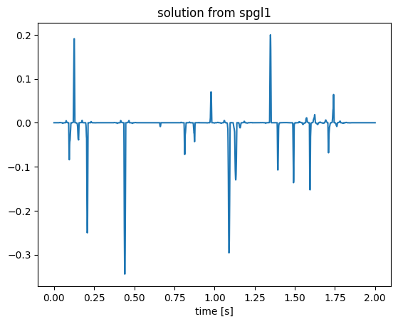
We can see that spgl1 produces a sparse solution as expected. Notice again that we did not provide a matrix to these algorithms, but "fooled" Julia by a JOLI linear operator equipped with forward and adjoint evaluations. lsqr and spgl1 algorithms work right away without any modification.
Automatic differentiation (AD) through the linear operator
Furthermore, we can follow the idea of ChainRules.jl package to "teach" Julia how to differentiate through the linear operators in JOLI---i.e., "teaches" Julia to apply the adjoint of the linear operator during back-propagation. With the efficient and effective abstraction, this can be done in less than 10 lines here. Taking advantage of this AD capability, we can solve the inverse problem with different regularization techniques and different objective functions. Since the gradient is provided by AD, we can use any kind of gradient-based optimization algorithm to acquire the solution. In the following example, we adopt a least-squares objective with an penalty as
and we use L-BFGS algorithm from Optim.jl package to iteratively invert the linear system. In this tutorial, we are not trying to find a best algorithm to solve this inverse problem, but demonstrating how JOLI works with different kinds of optimization schemes easily in a highly abstracted way.
λ = 1;   # weight on l1 regularization
loss(x) = .5 * norm(A * x - b)^2 + λ * norm(x,1);                 # objective function
δloss!(g, x) = begin g.=gradient(loss, x)[1]; return loss(x) end; # in-place gradient function
summary = optimize(loss, δloss!, zeros(N), LBFGS(), Optim.Options(iterations=500));
figure();plot(t, summary.minimizer);title("L-BFGS w/ 1-norm penalty");xlabel("time [s]");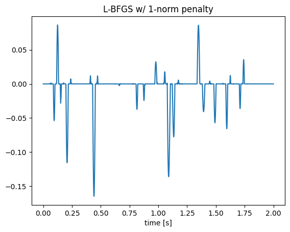
This AD capability also enables to expose JOLI linear operators to deep learning frameworks. To solve the inverse problem , we can reparameterize the input x by a network f with a fixed input z and solve for the network parameters instead---i.e.,
This is so-called deep prior approach discussed in Ulyanov, Dmitry, Andrea Vedaldi, and Victor Lempitsky. "Deep image prior." Proceedings of the IEEE conference on computer vision and pattern recognition. 2018. It has also been adopted into scientific computing and computational geoscience community, where A is PDE-based linear operator, such as in Siahkoohi, Ali, Gabrio Rizzuti, and Felix J. Herrmann. "Deep Bayesian inference for seismic imaging with tasks." arXiv preprint arXiv:2110.04825 (2021).
In this tutorial, we adopt a dense layer as a very simple deep prior network for demonstrative purpose only. In practice, the deep prior approach might need careful choices on the network structure and regularization parameters. Thanks to the abstraction, we can still write very clean code to interact with Flux and work with optimizers in Flux, such as ADAM.
f = Dense(2*N, N); # a very simple network
z = randn(2*N);    # fixed input
Flux.trainmode!(f, true);
θ = Flux.params(f);  # network parameters

# Optimizer
opt = ADAM(1f-4)
for j=1:500
    grads = gradient(θ) do
        return .5 * norm(A * f(z) - b)^2 + norm(f(z), 1) + norm(θ)^2;
    end

    # Update params
    for p in θ
        Flux.Optimise.update!(opt, p, grads[p])
    end
end
Flux.testmode!(f, true);
figure();plot(t, f(z));title("deep prior solution");xlabel("time [s]");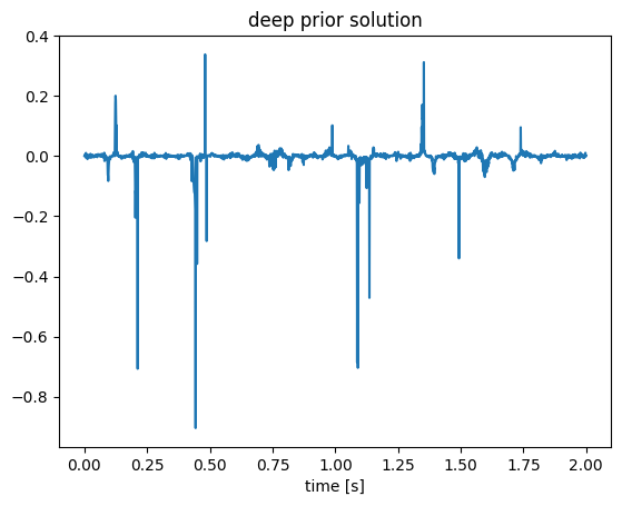
Thanks to the abstraction power of Julia, multiphysics data-driven framework can be written in a quite clean way in Julia, and can be inverted thanks to the AD capability. Another example of loop-unrolled seismic imaging with i-RIM network is documented in https://github.com/slimgroup/LoopUnrolledSeismicImaging, where the forward modeling operator is the linearized born modeing operator. You can find more applications of JOLI and the software abstraction idea at Louboutin, Mathias, et al. "Accelerating innovation with software abstractions for scalable computational geophysics." arXiv preprint arXiv:2203.15038 (2022).
You can also read the reference guide to learn more about JOLI in general. Issues and pull requests at the JOLI repository will also be highly appreciated!