Introduction to JUDI¶

JUDI.jl is a framework for large-scale seismic modeling and inversion and designed to enable rapid translations of algorithms to fast and efficient code that scales to industry-size 3D problems. The focus of the package lies on seismic modeling as well as PDE-constrained optimization such as full-waveform inversion (FWI) and imaging (LS-RTM). Wave equations in JUDI are solved with Devito, a Python domain-specific language for automated finite-difference (FD) computations. JUDI's modeling operators can also be used as layers in (convolutional) neural networks to implement physics-augmented deep learning algorithms. For this, check out JUDI's deep learning extension JUDI4Flux.

The JUDI software is published in Witte, Philipp A., et al. "A large-scale framework for symbolic implementations of seismic inversion algorithms in Julia." Geophysics 84.3 (2019): F57-F71.. For more information on usage of JUDI, you can check the JUDI reference guide.

This tutorial covers the following topics:

How to set up the geometry/acquisition in a seismic experiment
How software abstraction in Julia plays in role in the modeling via the abstracted linear operators
How to set up a mini-cluster to run seismic experiments parallel over shots

using JUDI, PyPlot, LinearAlgebra

Physical problem setup¶

Grid¶

JUDI relies on a cartesian grid for modeling and inversion. We start by defining the parameters needed for a cartesian grid:

A shape
A grid spacing in each direction
An origin

shape = (201, 201) # Number of gridpoints nx, nz
spacing = (10.0, 10.0) # in meters here
origin = (0.0, 0.0) # in meters as well

(0.0, 0.0)

Physical object¶

JUDI defines a few basic types to handle physical object such as the velocity model. The type PhyisicalParameter is an AbstractVector and behaves as a standard vector. A PhysicalParameter can be constructed in various ways but always require the origin o and grid spacing d that cannot be infered from the array.


    PhysicalParameter(v::Array{vDT}, d, o) where `v` is an n-dimensional array and n=size(v)

    PhysicalParameter(n, d, o; vDT=Float32) Creates a zero PhysicalParameter

    PhysicalParameter(v::Array{vDT}, A::PhysicalParameter) Creates a PhysicalParameter from the Array `v` with n, d, o from `A`

    PhysicalParameter(v::Array{vDT, N}, n::Tuple, d::Tuple, o::Tuple) where `v` is a vector or nd-array that is reshaped into shape `n`

    PhysicalParameter(v::vDT, n::Tuple, d::Tuple, o::Tuple) Creates a constant (single number) PhyicalParameter

Let's make a simple 3-layer velocity model

# Define the velocity (in km/s=m/ms)
vp = 1.5f0 * ones(Float32, shape)
vp[:, 66:end] .= 2.0f0
vp[:, 134:end] .= 2.5f0
# Create a physical parameter
VP = PhysicalParameter(vp, spacing, origin);

Let's plot the velocities. Because we adopt a standard cartesian dimension ordering for generality (X, Z) in 2D and (X, Y, Z) in 3D, we plot the transpose of the velocity for proper visualization.

figure(figsize=(12, 8));
subplot(121);
imshow(vp', cmap="jet", extent=[0, (shape[1]-1)*spacing[1], (shape[2]-1)*spacing[2], 0]);
xlabel("X [m]");ylabel("Depth [m]");
title("vp");
subplot(122);
imshow(VP', cmap="jet", extent=[0, (shape[1]-1)*spacing[1], (shape[2]-1)*spacing[2], 0]);
xlabel("X [m]");ylabel("Depth [m]");
title("vp as a physical parameter");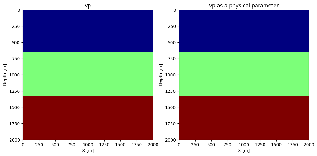

Figure(PyObject <Figure size 1200x800 with 2 Axes>)

Because the physical parameter behaves as vector, we can easily perform standard operations on it.

norm(VP), extrema(VP), 2f0 .* VP, VP .^ 2

(411.6956f0, (1.5f0, 2.5f0), PhysicalParameter{Float32} of size (201, 201) with origin (0.0, 0.0) and spacing (10.0, 10.0), PhysicalParameter{Float32} of size (201, 201) with origin (0.0, 0.0) and spacing (10.0, 10.0))

Model¶

JUDI then provide a Model structure that wraps multiple physical parameters together.

model = Model(shape, spacing, origin, 1f0./vp.^2f0; nb = 80)

Model (n=(201, 201), d=(10.0, 10.0), o=(0.0, 0.0)) with parameters [:m]

Modeling¶

Now that we have a seismic model, we will generate a few shot records.

Acquisition Geometry¶

The first thing we need is an acquisiton geometry. In JUDI, there are two ways to create a Geometry.

By hand, as we will show here
From a SEGY file, as we will show in a follow-up tutorial

We create a split-spread geomtry with sources at the top and receivers at the ocean bottom (top of second layer).

Note:

For 2D simulation (i.e. wave propagation in a 2D plane), JUDI still takes y-coordinate of source/receiver locations but we can just put them to 0 anyway.

# Sources position
nsrc = 11
xsrc = range(0f0, (shape[1] -1)*spacing[1], length=nsrc)
ysrc = 0f0 .* xsrc # this a 2D case so we set y to 0
zsrc = 12.5f0*ones(Float32, nsrc);

Now this definition creates a single Array of position, which would correspond to a single simultenous source (firing at the same time). Since we are interested in single source experiments here, we convert these position into an Array of Array of size nsrc where each sub-array is a single source position

xsrc, ysrc, zsrc = convertToCell.([xsrc, ysrc, zsrc]);

# OBN position
nrec = 101
xrec = range(0f0, (shape[1] -1)*spacing[1], length=nrec)
yrec = 0f0 # this a 2D case so we set y to 0. This can be a single number for receivers
zrec = (66*spacing[1])*ones(Float32, nrec);

The last step to be able to create and acquisiton geometry is to define a recording time and sampling rate

record_time = 2000f0 # Recording time in ms (since we have m/ms for the velocity)
sampling_rate = 4f0; # Let's use a standard 4ms sampling rate

Now we can create the source and receivers geometry

src_geom = Geometry(xsrc, ysrc, zsrc; dt=sampling_rate, t=record_time)
# For the receiver geometry, we specify the number of source to tell JUDI to use the same receiver position for all sources
rec_geom = Geometry(xrec, yrec, zrec, dt=sampling_rate, t=record_time, nsrc=nsrc);

Let's visualize the geometry onto the model

figure();
imshow(vp', cmap="jet", extent=[0, (shape[1]-1)*spacing[1], (shape[2]-1)*spacing[2], 0]);
scatter(xsrc, zsrc, label=:sources);
scatter(xrec, zrec, label="OBN");
xlabel("X [m]");ylabel("Depth [m]");
legend();
title("acquisition geometry")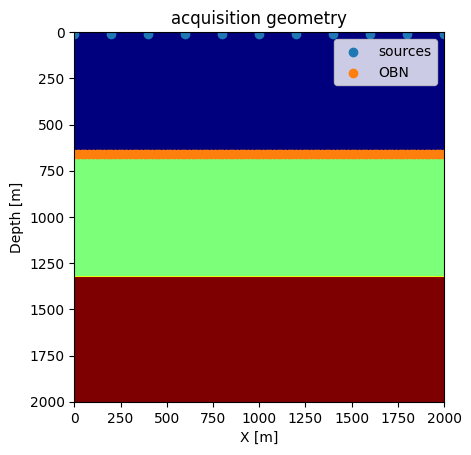

Figure(PyObject <Figure size 640x480 with 1 Axes>)

PyObject Text(0.5, 1.0, 'acquisition geometry')

Source wavelet¶

For the source wavelet, we will use a standard Ricker wavelet at 10Hz for this tutorial. In practice, this wavelet would be read from a file or estimated during inversion.

f0 = 0.010 # Since we use ms, the frequency is in KHz
wavelet = ricker_wavelet(record_time, sampling_rate, f0);
plot(wavelet)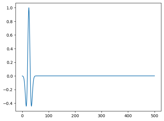

1-element Vector{PyCall.PyObject}:
 PyObject <matplotlib.lines.Line2D object at 0x7ff48ef2cad0>

judiVector¶

In order to represent seismic data, JUDI provide the judiVector type. This type wraps a geometry with the seismic data corresponding to it. Note that judiVector works for both shot records at the receiver locations and for the wavelet at the source locations. Let's create one for the source

q = judiVector(src_geom, wavelet)

judiVector{Float32, Matrix{Float32}} with 11 sources

Linear operator¶

Following the math, the seismic data recorded at the receiver locations can be calculated by

\mathbf{d}_{obs} = \mathbf{P}_r \mathbf{A}(\mathbf{m})^{-1} \mathbf{P}_s^{\top}\mathbf{q},

(1)

Here, $\mathbf{q}$ is the source wavelet set up at the firing locations (defined above). $\mathbf{P}_s^{\top}$ injects $\mathbf{q}$ to the entire space. $\mathbf{A}(\mathbf{m})$ is the discretized wave equation parameterized by squared slowness $\mathbf{m}$ . By applying the inverse of $\mathbf{A}(\mathbf{m})$ on source $\mathbf{q}$ , we acquire the entire wavefield in the space. Finally, $\mathbf{P}_r$ restricts the wavefield at the receiver locations at the recording time.

Now let's these linear operators, which behave as "matrices".

Pr = judiProjection(rec_geom) # receiver interpolation

judiProjection{Float32}(AbstractSize(Dict{Symbol, Any}(:src => 11, :rec => [101, 101, 101, 101, 101, 101, 101, 101, 101, 101, 101], :time => Integer[501, 501, 501, 501, 501, 501, 501, 501, 501, 501, 501])), AbstractSize(Dict{Symbol, Any}(:x => 0, :src => 11, :y => 0, :z => 0, :time => Integer[501, 501, 501, 501, 501, 501, 501, 501, 501, 501, 501])), GeometryIC{Float32} wiht 11 sources)

Ps = judiProjection(src_geom) # Source interpolation

judiProjection{Float32}(AbstractSize(Dict{Symbol, Any}(:src => 11, :rec => [1, 1, 1, 1, 1, 1, 1, 1, 1, 1, 1], :time => Integer[501, 501, 501, 501, 501, 501, 501, 501, 501, 501, 501])), AbstractSize(Dict{Symbol, Any}(:x => 0, :src => 11, :y => 0, :z => 0, :time => Integer[501, 501, 501, 501, 501, 501, 501, 501, 501, 501, 501])), GeometryIC{Float32} wiht 11 sources)

Ainv = judiModeling(model) # Inverse of the disrete ewave equation

JUDI forward{Float32} propagator (x * z * time) -> (x * z * time)

WARNING While these three operator are well defined in JUDI, judiProjection is a no-op operator and cannot be used by itself but only in combination with a judiModeling operator

Seismic data generation¶

With the set-up operators above, we can finally generate synthetic data with simple mat-vec product thanks to the abstraction.

d_obs = Pr * Ainv * Ps' * q

Operator `forward` ran in 0.21 s
Operator `forward` ran in 0.21 s
Operator `forward` ran in 0.21 s
Operator `forward` ran in 0.21 s
Operator `forward` ran in 0.21 s
Operator `forward` ran in 0.21 s
Operator `forward` ran in 0.21 s
Operator `forward` ran in 0.21 s
Operator `forward` ran in 0.21 s
Operator `forward` ran in 0.22 s
Operator `forward` ran in 0.21 s

judiVector{Float32, Matrix{Float32}} with 11 sources

Similarly, we can define a modeling operator F that combines the modeling operator with source/receiver restriction operators, as

F = Pr * Ainv * Ps'

JUDI forward{Float32} propagator (src * rec * time) -> (src * rec * time)

We can run the same code to generate the data

d_obs = F * q

Operator `forward` ran in 0.21 s
Operator `forward` ran in 0.21 s
Operator `forward` ran in 0.21 s
Operator `forward` ran in 0.21 s
Operator `forward` ran in 0.21 s
Operator `forward` ran in 0.21 s
Operator `forward` ran in 0.21 s
Operator `forward` ran in 0.21 s
Operator `forward` ran in 0.22 s
Operator `forward` ran in 0.21 s
Operator `forward` ran in 0.21 s

judiVector{Float32, Matrix{Float32}} with 11 sources

There are 11 sources in this experiment, and the data is generated for each shot independently. If we only want to acquire the data for the 6th source for example, then we can run

d_obs6 = F[6] * q[6]

Operator `forward` ran in 0.22 s

judiVector{Float32, Matrix{Float32}} with 1 sources

data_extent = [xrec[1], xrec[end], 1f-3*record_time, 0]
figure(figsize=(20, 5))
for i=1:5
    subplot(1, 5, i)
    imshow(d_obs.data[2*i], vmin=-1, vmax=1, cmap="Greys", extent=data_extent, aspect="auto")
    xlabel("Receiver position (m)")
    ylabel("Recording time (s)")
    title("xsrc=$(1f-3xsrc[2*i][1])km")
end
tight_layout()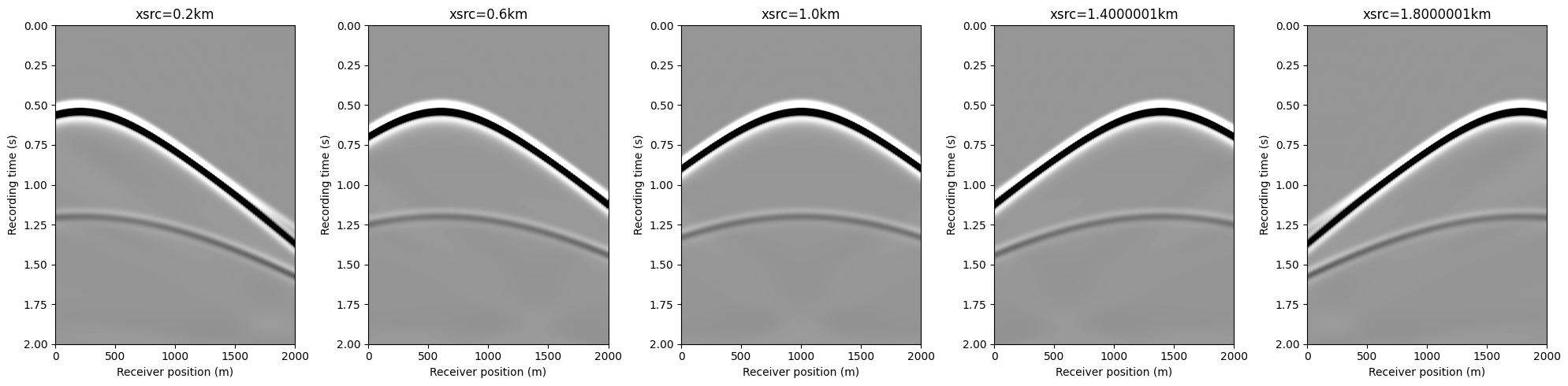

Figure(PyObject <Figure size 2000x500 with 5 Axes>)

Parallelization -- workers and threads¶

JUDI (based on Devito) uses shared memory OpenMP parallelism for solving PDEs. Here, we show how to build up a small 2-worker cluster by calling addprocs(2). Because we set the environment variable ENV["OMP_DISPLAY_ENV"] = "true", we will see the OMP environment printed out on each worker.

We set 4 environment variables related to OpenMP:

OMP_DISPLAY_ENV prints out the OpenMP environment on each worker
OMP_PROC_BIND specifies that threads should be bound to physical cores
OMP_NUM_THREADS specifies the number of threads per workers is 1/nw the number of physical cores
GOMP_CPU_AFFINITY specifies which physical cores the threads run on for each worker

If you run the shell command top during execution, you will see 3 julia processes: the main process and 2 workers. The two workers should generally have about 50% of the system, and load average should tend towards the physical number of cores. When running with multiple workers, we gain the parallelism over sources.

using Distributed

# Sytem informations
nthread = Sys.CPU_THREADS
nw = 2

ENV["OMP_DISPLAY_ENV"] = "true"
ENV["OMP_PROC_BIND"] = "close"
ENV["OMP_NUM_THREADS"] = "$(div(nthread, nw))"
addprocs(nw; lazy=false)
@show workers()
for k in 1:nworkers()
    place1 = (k - 1) * div(nthread,nworkers())
    place2 = (k + 0) * div(nthread,nworkers()) - 1
    @show place1, place2, div(nthread, nw)
    @spawnat workers()[k] ENV["GOMP_CPU_AFFINITY"] = "$(place1)-$(place2)";
end

@everywhere using Distributed
@everywhere using JUDI

workers() = [2, 3]
(place1, place2, div(nthread, nw)) = (0, 5, 6)
(place1, place2, div(nthread, nw)) = (6, 11, 6)
      From worker 3:	
      From worker 3:	OPENMP DISPLAY ENVIRONMENT BEGIN
      From worker 3:	  _OPENMP = '201511'
      From worker 3:	  OMP_DYNAMIC = 'FALSE'
      From worker 3:	  OMP_NESTED = 'FALSE'
      From worker 3:	  OMP_NUM_THREADS = '6'
      From worker 3:	  OMP_SCHEDULE = 'DYNAMIC'
      From worker 3:	  OMP_PROC_BIND = 'CLOSE'
      From worker 3:	  OMP_PLACES = ''
      From worker 3:	  OMP_STACKSIZE = '2097152'
      From worker 3:	  OMP_WAIT_POLICY = 'PASSIVE'
      From worker 3:	  OMP_THREAD_LIMIT = '4294967295'
      From worker 3:	  OMP_MAX_ACTIVE_LEVELS = '1'
      From worker 3:	  OMP_CANCELLATION = 'FALSE'
      From worker 3:	  OMP_DEFAULT_DEVICE = '0'
      From worker 3:	  OMP_MAX_TASK_PRIORITY = '0'
      From worker 3:	  OMP_DISPLAY_AFFINITY = 'FALSE'
      From worker 3:	  OMP_AFFINITY_FORMAT = 'level %L thread %i affinity %A'
      From worker 3:	  OMP_ALLOCATOR = 'omp_default_mem_alloc'
      From worker 3:	  OMP_TARGET_OFFLOAD = 'DEFAULT'
      From worker 3:	OPENMP DISPLAY ENVIRONMENT END
      From worker 2:	
      From worker 2:	OPENMP DISPLAY ENVIRONMENT BEGIN
      From worker 2:	  _OPENMP = '201511'
      From worker 2:	  OMP_DYNAMIC = 'FALSE'
      From worker 2:	  OMP_NESTED = 'FALSE'
      From worker 2:	  OMP_NUM_THREADS = '6'
      From worker 2:	  OMP_SCHEDULE = 'DYNAMIC'
      From worker 2:	  OMP_PROC_BIND = 'CLOSE'
      From worker 2:	  OMP_PLACES = ''
      From worker 2:	  OMP_STACKSIZE = '2097152'
      From worker 2:	  OMP_WAIT_POLICY = 'PASSIVE'
      From worker 2:	  OMP_THREAD_LIMIT = '4294967295'
      From worker 2:	  OMP_MAX_ACTIVE_LEVELS = '1'
      From worker 2:	  OMP_CANCELLATION = 'FALSE'
      From worker 2:	  OMP_DEFAULT_DEVICE = '0'
      From worker 2:	  OMP_MAX_TASK_PRIORITY = '0'
      From worker 2:	  OMP_DISPLAY_AFFINITY = 'FALSE'
      From worker 2:	  OMP_AFFINITY_FORMAT = 'level %L thread %i affinity %A'
      From worker 2:	  OMP_ALLOCATOR = 'omp_default_mem_alloc'
      From worker 2:	  OMP_TARGET_OFFLOAD = 'DEFAULT'
      From worker 2:	OPENMP DISPLAY ENVIRONMENT END

d_obs = F * q

      From worker 2:	
      From worker 2:	OPENMP DISPLAY ENVIRONMENT BEGIN
      From worker 2:	  _OPENMP = '201511'
      From worker 2:	  OMP_DYNAMIC = 'FALSE'
      From worker 2:	  OMP_NESTED = 'FALSE'
      From worker 2:	  OMP_NUM_THREADS = '6'
      From worker 2:	  OMP_SCHEDULE = 'DYNAMIC'
      From worker 2:	  OMP_PROC_BIND = 'CLOSE'
      From worker 2:	  OMP_PLACES = ''
      From worker 2:	  OMP_STACKSIZE = '2097152'
      From worker 2:	  OMP_WAIT_POLICY = 'PASSIVE'
      From worker 2:	  OMP_THREAD_LIMIT = '4294967295'
      From worker 2:	  OMP_MAX_ACTIVE_LEVELS = '2147483647'
      From worker 2:	  OMP_CANCELLATION = 'FALSE'
      From worker 2:	  OMP_DEFAULT_DEVICE = '0'
      From worker 2:	  OMP_MAX_TASK_PRIORITY = '0'
      From worker 2:	OPENMP DISPLAY ENVIRONMENT END
      From worker 3:	
      From worker 3:	OPENMP DISPLAY ENVIRONMENT BEGIN
      From worker 3:	  _OPENMP = '201511'
      From worker 3:	  OMP_DYNAMIC = 'FALSE'
      From worker 3:	  OMP_NESTED = 'FALSE'
      From worker 3:	  OMP_NUM_THREADS = '6'
      From worker 3:	  OMP_SCHEDULE = 'DYNAMIC'
      From worker 3:	  OMP_PROC_BIND = 'CLOSE'
      From worker 3:	  OMP_PLACES = ''
      From worker 3:	  OMP_STACKSIZE = '2097152'
      From worker 3:	  OMP_WAIT_POLICY = 'PASSIVE'
      From worker 3:	  OMP_THREAD_LIMIT = '4294967295'
      From worker 3:	  OMP_MAX_ACTIVE_LEVELS = '2147483647'
      From worker 3:	  OMP_CANCELLATION = 'FALSE'
      From worker 3:	  OMP_DEFAULT_DEVICE = '0'
      From worker 3:	  OMP_MAX_TASK_PRIORITY = '0'
      From worker 3:	OPENMP DISPLAY ENVIRONMENT END
      From worker 2:	Operator `forward` ran in 0.27 s
      From worker 3:	Operator `forward` ran in 0.26 s
      From worker 2:	Operator `forward` ran in 0.28 s
      From worker 3:	Operator `forward` ran in 0.28 s
      From worker 2:	Operator `forward` ran in 0.29 s
      From worker 3:	Operator `forward` ran in 0.29 s
      From worker 2:	Operator `forward` ran in 0.21 s
      From worker 3:	Operator `forward` ran in 0.23 s
      From worker 2:	Operator `forward` ran in 0.22 s
      From worker 3:	Operator `forward` ran in 0.23 s
      From worker 2:	Operator `forward` ran in 0.21 s

judiVector{Float32, Matrix{Float32}} with 11 sources

Reverse time migration¶

Reverse time migration (RTM) is a seismic migration method to move the dipping events in the data domain to their supposedly true subsurface positions in the image domain. This is also a linear operation, as shown in our abstraction below.

J = judiJacobian(F, q)    # forward is linearized born modeling, adjoint is reverse time migration
rtm = J' * d_obs

      From worker 2:	Operator `forward` ran in 0.22 s
      From worker 3:	Operator `forward` ran in 0.32 s
      From worker 2:	Operator `gradient` ran in 0.33 s
      From worker 3:	Operator `gradient` ran in 0.27 s
      From worker 2:	Operator `forward` ran in 0.23 s
      From worker 3:	Operator `forward` ran in 0.32 s
      From worker 2:	Operator `gradient` ran in 0.35 s
      From worker 3:	Operator `gradient` ran in 0.27 s
      From worker 2:	Operator `forward` ran in 0.25 s
      From worker 3:	Operator `forward` ran in 0.30 s
      From worker 2:	Operator `gradient` ran in 0.32 s
      From worker 3:	Operator `gradient` ran in 0.27 s
      From worker 2:	Operator `forward` ran in 0.24 s
      From worker 3:	Operator `forward` ran in 0.29 s
      From worker 2:	Operator `gradient` ran in 0.32 s
      From worker 3:	Operator `gradient` ran in 0.28 s
      From worker 2:	Operator `forward` ran in 0.23 s
      From worker 3:	Operator `forward` ran in 0.28 s
      From worker 2:	Operator `gradient` ran in 0.31 s
      From worker 3:	Operator `gradient` ran in 0.24 s
      From worker 3:	Operator `forward` ran in 0.22 s
      From worker 3:	Operator `gradient` ran in 0.24 s

PhysicalParameter{Float32} of size (201, 201) with origin (0.0, 0.0) and spacing (10.0, 10.0)

figure();
imshow(rtm', cmap="Greys", extent=[0, (shape[1]-1)*spacing[1], (shape[2]-1)*spacing[2], 0]);
xlabel("X [m]");ylabel("Depth [m]");
title("RTM");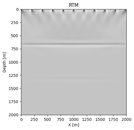

References¶

Witte, P. A., Louboutin, M., Kukreja, N., Luporini, F., Lange, M., Gorman, G. J., & Herrmann, F. J. (2019). A large-scale framework for symbolic implementations of seismic inversion algorithms in Julia. GEOPHYSICS, 84(3), F57–F71. 10.1190/geo2018-0174.1

Notebooks

Linear algebra abstractions in JOLI.jl

Notebooks

SEGY handling in SegyIO.jl