Inversions
In this notebook, we use a synthetic example to explore aspects of inversion including:
- assigning uncertainties to the the data
- adjusting the regularization parameters on the smallness and smoothness terms
- adjusting the value of the trade-off parameter
Step 0: Imports and load survey info
These steps are the same as in the previous notebook.
# core python
import numpy as np
import matplotlib.pyplot as plt
from matplotlib.colors import LogNorm, SymLogNorm, Normalize
import matplotlib.gridspec as gridspec
import ipywidgets

# tools in the simPEG Ecosystem
import discretize  # for creating computational meshes

# linear solvers
try:
    from pymatsolver import Pardiso as Solver  # this is a fast linear solver
except ImportError:
    from SimPEG import SolverLU as Solver  # this will be slower

# SimPEG inversion machinery
from SimPEG import (
    Data, maps,
    data_misfit, regularization, optimization, inverse_problem,
    inversion, directives
)

# DC resistivity and IP modules
from SimPEG.electromagnetics import resistivity as dc
# set the font size in the plots
from matplotlib import rcParams
rcParams["font.size"] = 14try:
import warnings
warnings.filterwarnings('ignore')
except:
passStep 1: Load DC Survey
This is the same as in the previous notebook, but included so we can re-visit any of the steps as necessary.
line = "46800E"

dc_data_file = f"./century/{line}/{line[:-1]}POT.OBS"
def read_dcip_data(filename, verbose=True):
"""
Read in a .OBS file from the Century data set into a python dictionary.
The format is the old UBC-GIF DCIP format.
Parameters
----------
filename : str
Path to the file to be parsed
verbose: bool
Print some things?
Returns
-------
dict
A dictionary with the locations of
- a_locations: the positive source electrode locations (numpy array)
- b_locations: the negative source electrode locations (numpy array)
- m_locations: the receiver locations (list of numpy arrays)
- n_locations: the receiver locations (list of numpy arrays)
- n_locations: the receiver locations (list of numpy arrays)
- observed_data: observed data (list of numpy arrays)
- standard_deviations: assigned standard deviations (list of numpy arrays)
- n_sources: number of sources (int)
"""
# read in the text file as a numpy array of strings (each row is an entry)
contents = np.genfromtxt(filename, delimiter=' \n', dtype=np.str)
# the second line has the number of sources, current, and data type (voltages if 1)
n_sources = int(contents[1].split()[0])
if verbose is True:
print(f"number of sources: {n_sources}")
# initialize storage for the electrode locations and data
a_locations = np.zeros(n_sources)
b_locations = np.zeros(n_sources)
m_locations = []
n_locations = []
observed_data = []
standard_deviations = []
# index to track where we have read in content
content_index = 1
# loop over sources
for i in range(n_sources):
# start by reading in the source info
content_index = content_index + 1 # read the next line
a_location, b_location, nrx = contents[content_index].split() # this is a string
# convert the strings to a float for locations and an int for the number of receivers
a_locations[i] = float(a_location)
b_locations[i] = float(b_location)
nrx = int(nrx)
if verbose is True:
print(f"Source {i}: A-loc: {a_location}, B-loc: {b_location}, N receivers: {nrx}")
# initialize space for receiver locations, observed data associated with this source
m_locations_i, n_locations_i = np.zeros(nrx), np.zeros(nrx)
observed_data_i, standard_deviations_i = np.zeros(nrx), np.zeros(nrx)
# read in the receiver info
for j in range(nrx):
content_index = content_index + 1 # read the next line
m_location, n_location, datum, std = contents[content_index].split()
# convert the locations and data to floats, and store them
m_locations_i[j] = float(m_location)
n_locations_i[j] = float(n_location)
observed_data_i[j] = float(datum)
standard_deviations_i[j] = float(std)
# append the receiver info to the lists
m_locations.append(m_locations_i)
n_locations.append(n_locations_i)
observed_data.append(observed_data_i)
standard_deviations.append(standard_deviations_i)
return {
"a_locations": a_locations,
"b_locations": b_locations,
"m_locations": m_locations,
"n_locations": n_locations,
"observed_data": observed_data,
"standard_deviations": standard_deviations,
"n_sources": n_sources,
}dc_data_dict = read_dcip_data(dc_data_file, verbose=False)# initialize an empty list for each
source_list = []
# center the survey and work in local coordinates
x_local = 0.5*(np.min(dc_data_dict["a_locations"]) + np.max(np.hstack(dc_data_dict["n_locations"])))
for i in range(dc_data_dict["n_sources"]):
# receiver electrode locations in 2D
m_locs = np.vstack([
dc_data_dict["m_locations"][i] - x_local,
np.zeros_like(dc_data_dict["m_locations"][i])
]).T
n_locs = np.vstack([
dc_data_dict["n_locations"][i] - x_local,
np.zeros_like(dc_data_dict["n_locations"][i])
]).T
# construct the receiver object
receivers = dc.receivers.Dipole(locations_m=m_locs, locations_n=n_locs, storeProjections=False)
# construct the source
source = dc.sources.Dipole(
location_a=np.r_[dc_data_dict["a_locations"][i] - x_local, 0.],
location_b=np.r_[dc_data_dict["b_locations"][i] - x_local, 0.],
receiver_list=[receivers]
)
# append the new source to the source list
source_list.append(source)survey = dc.Survey(source_list=source_list)Step 2: Build a Mesh
Similar to the previous notebook, we use a simple function to design our mesh.
def build_mesh(
    survey=survey,
    n_cells_per_spacing_x=4,
    n_cells_per_spacing_z=4,
    n_core_extra_x=4,
    n_core_extra_z=4,
    core_domain_z_ratio=1/3.,
    padding_factor=1.3,
    n_pad_x=10,
    n_pad_z=10,
):
    """
    A function for designing a Tensor Mesh based on DC survey parameters

    Parameters
    ----------

    survey: dc.Survey
        A DC (or IP) survey object

    n_cells_per_spacing_[x, z]: int
        Number of [x, z]-cells per the minimum electrode spacing

    n_core_extra_[x, z]: int
        Number of extra cells with the same size as the core domain beyond the survey extent

    core_domain_z_ratio: float
        Factor that multiplies the maximum AB, MN separation to define the core mesh extent

    padding_factor: float
        Factor by which we expand the mesh cells in the padding region

    n_pad_[x, z]: int
        Number of padding cells in the x, z directions
    """
    min_electrode_spacing = np.min(np.abs(survey.locations_a[:, 0] - survey.locations_b[:, 0]))

    dx = min_electrode_spacing / n_cells_per_spacing_x
    dz = min_electrode_spacing / n_cells_per_spacing_z

    # define the x core domain
    core_domain_x = np.r_[
        survey.electrode_locations[:, 0].min(),
        survey.electrode_locations[:, 0].max()
    ]

    # find the y core domain
    # find the maximum spacing between source, receiver midpoints
    mid_ab = (survey.locations_a + survey.locations_b)/2
    mid_mn = (survey.locations_m + survey.locations_n)/2
    separation_ab_mn = np.abs(mid_ab - mid_mn)
    max_separation = separation_ab_mn.max()
    core_domain_z = np.r_[-core_domain_z_ratio * max_separation, 0.]

    # add extra cells beyond the core domain
    n_core_x = np.ceil(np.diff(core_domain_x)/dx) + n_core_extra_x*2  # on each side
    n_core_z = np.ceil(np.diff(core_domain_z)/dz) + n_core_extra_z  # just below

    # define the tensors in each dimension
    hx = [(dx, n_pad_x, -padding_factor), (dx, n_core_x), (dx, n_pad_x, padding_factor)]
    hz = [(dz, n_pad_z, -padding_factor), (dz, n_core_z)]

    mesh = discretize.TensorMesh([hx, hz], x0="CN")

    return mesh, core_domain_x, core_domain_z
mesh, core_domain_x, core_domain_z = build_mesh(survey)
mesh.plotGrid()<AxesSubplot:xlabel='x1', ylabel='x2'>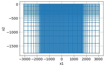
Step 3: Design our True Model
Here, we will focus in on a synthetic example so we know the true solution. Again, we will use a model containing 2 blocks in a halfspace.
3.1 Define the model geometry and physical properties
Here, we define a model with one conductive block and one resistive block in a halfspace.
# define the resistivities
rho_background = 100
rho_resistive_block = 1000
rho_conductive_block = 10

# define the geometry of each block
xlim_resistive_block = np.r_[-500, -250]
zlim_resistive_block = np.r_[-150, -75]

xlim_conductive_block = np.r_[250, 500]
zlim_conductive_block = np.r_[-150, -75]
rho = rho_background * np.ones(mesh.nC)
# resistive block
inds_resistive_block = (
(mesh.gridCC[:, 0] >= xlim_resistive_block.min()) & (mesh.gridCC[:, 0] <= xlim_resistive_block.max()) &
(mesh.gridCC[:, 1] >= zlim_resistive_block.min()) & (mesh.gridCC[:, 1] <= zlim_resistive_block.max())
)
rho[inds_resistive_block] = rho_resistive_block
# conductive block
inds_conductive_block = (
(mesh.gridCC[:, 0] >= xlim_conductive_block.min()) & (mesh.gridCC[:, 0] <= xlim_conductive_block.max()) &
(mesh.gridCC[:, 1] >= zlim_conductive_block.min()) & (mesh.gridCC[:, 1] <= zlim_conductive_block.max())
)
rho[inds_conductive_block] = rho_conductive_blockfig, ax = plt.subplots(1, 1, figsize=(12, 4))
out = mesh.plotImage(np.log10(rho), ax=ax, pcolorOpts={"cmap":"Spectral"})
plt.colorbar(out[0], ax=ax, label="log$_{10} \\rho$", orientation="horizontal", fraction=0.05, pad=0.25)
ax.set_xlim(core_domain_x)
ax.set_ylim(core_domain_z + np.r_[-100, 0])
ax.set_aspect(1.5)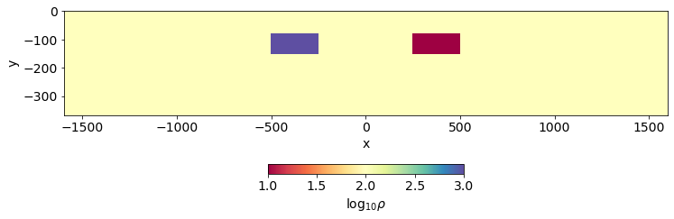
3.2 Define the true model
Since we will be working with log-resistivities in the inversion, our true model is defined as the log of the resistivity.
model_true = np.log(rho)Step 4: Set up and run a forward simulation
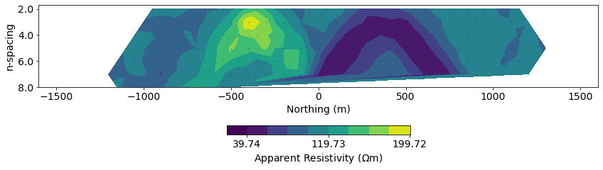
These will be the "observed data" in the inversion. We add noise to the result (a default of 5%). If you would like to adjust the noise level, you can change the relative_error, you can pass add_noise to the make_synthetic_data function.
As in the first notebook, we will invert for log-resistivity, so we use an ExpMap in the forward simulation. Again, we use the storeJ option to store the
mapping = maps.ExpMap(mesh)

# Generate 2.5D DC problem
simulation_dc = dc.Simulation2DNodal(
    mesh, rhoMap=mapping, solver=Solver, survey=survey, storeJ=True
)
%%time
# compute our "observed data"
synthetic_data = simulation_dc.make_synthetic_data(model_true, add_noise=True)CPU times: user 1.01 s, sys: 77.2 ms, total: 1.09 s
Wall time: 373 ms
# plot pseudosections
fig, ax = plt.subplots(1, 1, figsize=(12, 4))

# plot a psuedosection of the data
dc.utils.plot_pseudosection(
    synthetic_data, data_type="apparent resistivity",
    plot_type="contourf", data_location=True, ax=ax,
    cbar_opts={"pad":0.25}
)
ax.set_xlim(core_domain_x)
ax.set_aspect(1.5)  # some vertical exxageration
ax.set_xlabel("Northing (m)")

plt.tight_layout()
Recall: inversion as optimization
We forumlate the inverse problem as an optimization problem consisting of a data misfit and a regularization
where:
is our inversion model - a vector containing the set of parameters that we invert for
is the data misfit
is the regularization
is a trade-off parameter that weights the relative importance of the data misfit and regularization terms
is our target misfit, which is typically set to where is the number of data (Parker, 1994) (or also see Oldenburg & Li (2005))
Step 5: assign standard deviations to the data
The standard deviations are an estimate of the level of noise on your data. These are used to construct the weights in the matrix of the data misfit.
It is common to define the standard deviation in terms of a relative_error and a noise_floor.
KaTeX parse error: Expected 'EOF', got '_' at position 15: \text{standard_̲deviation} =  \…

\text{standard_deviation} =  \text{relative_error}\times|d^{obs}| + \text{noise_floor}
For DC resistivity, it is common to choose a relative_error between 0.02-0.1 (2% - 10% error). The noise_floor value defines threshold for data below which we consider those values to be close to zero. It is important to set a non-zero noise_floor when we can have zero-crossings in our data (e.g. both positive and negative values - which we do in DC!). The noise_floor ensures that we don't try to fit near-zero values to very high accuracy.
fig, ax = plt.subplots(1, 1)
ax.hist(np.log10(np.abs(synthetic_data.dobs)), 30)
ax.set_xlabel("$log_{10}(|d^{obs}|)$")
Text(0.5, 0, '$log_{10}(|d^{obs}|)$')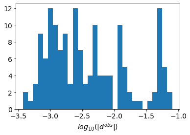
relative_error = 0.05  # 5% error
noise_floor = 1e-4
fig, ax = plt.subplots(1, 1)
ax.hist(np.log10(np.abs(synthetic_data.dobs)), 30)
ax.set_xlabel("$log_{10}(|d^{obs}|)$")
ax.axvline(np.log10(noise_floor), linestyle="dashed", color="C1")<matplotlib.lines.Line2D at 0x12bbe1750>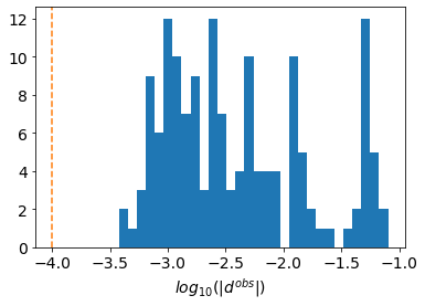
5.1 Assign uncertainties to our data object
In SimPEG, the data object is responsible for keeping track of the survey geometry, observed data and uncertainty values. The standard_deviation property is what is used to construct the matrix in the data misfit
W_d = diag(1 / data.standard_deviation) synthetic_data.relative_error = relative_error
synthetic_data.noise_floor = noise_floorassert(np.allclose(
relative_error * np.abs(synthetic_data.dobs) + noise_floor,
synthetic_data.standard_deviation
))Plot the data sorted by amplitude and associated uncertainties.
inds_sort = np.argsort(np.abs(synthetic_data.dobs))
sorted_data = np.abs(synthetic_data.dobs[inds_sort])
sorted_std = synthetic_data.standard_deviation[inds_sort]
fig, ax = plt.subplots(2, 1, figsize=(12, 8))
x = np.arange(0, len(sorted_data))
ax[0].plot(x, sorted_data, '.k')
ax[1].semilogy(x, sorted_data, '.k')
ax[0].set_title("sorted data and associated uncertainties")
for a in ax:
a.fill_between(x, sorted_data - sorted_std, sorted_data + sorted_std, alpha=0.25)
a.grid(alpha=0.5)
a.set_ylabel("observed data (V)")
plt.tight_layout()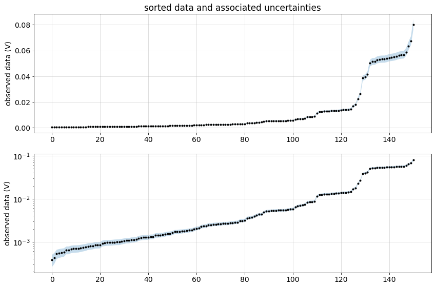
Step 6: Assembling the inversion
Here, we are going to set up functions for constructing and running the inversion so that we can easily adjust the parameters used in the inversion.
We start be defining a function that will construct our inverse_problem object which requires the data_misfit, regularization, and optimization be constructed.
def create_inverse_problem(
relative_error=relative_error, noise_floor=noise_floor,
alpha_s=1e-3, alpha_x=1, alpha_z=1, mref=np.log(rho_background),
maxIter=20, maxIterCG=20,
):
"""
A function that contructs a data misfit, regularization, and optimization and
assembles them into an inverse_problem object.
Parameters
----------
relative_error: float
relative error we assign to the data (used to construct the standard_deviation)
noise_floor: float
noise floor that we use to construct the standard deviations of the data
alpha_s: float
weight for the smallness component of the regularization
alpha_[x, z]: float
weight for the [x, z]-smoothness term in the regularization
mref: float
reference model value used in the smallness term of the regularization
maxIter: int
maximum number of iterations in the inversion
maxIterCG: int
maximum number of Conjugate Gradient iterations used to compute a step
in the Inexact Gauss Newton optimization
"""
# set the uncertainties and define the data misfit
synthetic_data.relative_error = relative_error
synthetic_data.noise_floor = noise_floor
dmisfit = data_misfit.L2DataMisfit(data=synthetic_data, simulation=simulation_dc)
# regularization
reg = regularization.Tikhonov(
mesh, alpha_s=alpha_s, alpha_x=alpha_x, alpha_y=alpha_z, mref=mref*np.ones(mesh.nC)
)
# optimization
opt = optimization.InexactGaussNewton(maxIter=maxIter, maxIterCG=maxIterCG)
opt.remember("xc")
# return the inverse problem
return inverse_problem.BaseInvProblem(dmisfit, reg, opt)Next, we define a simple function for assembling the inversion. There are very simiar functions in SimPEG already that write these outputs to a file (see for example directives.SaveOutputEveryIteration). In part, I show this here to give you a sense of how directives work in the inversion so if you are interested in writing your own, then you can use this as a template.
The initialize method is called at the very beginning of the inversion. In the BetaEstimate_ByEig, which we used in notebook 1, this is where we initialze an estimate of beta.
The endIter method is called at the end of every iteration. For example in the BetaSchedule directive, this is where we update the value of beta.
In this directive, we will create a simple dictionary that saves some outputs of interest during the inversion.
class SaveInversionProgress(directives.InversionDirective):
    """
    A custom directive to save items of interest during the course of an inversion
    """

    def initialize(self):
        """
        This is called when we first start running an inversion
        """
        # initialize an empty dictionary for storing results
        self.inversion_results = {
            "iteration":[],
            "beta":[],
            "phi_d":[],
            "phi_m":[],
            "phi_m_small":[],
            "phi_m_smooth_x":[],
            "phi_m_smooth_z":[],
            "dpred":[],
            "model":[]
        }

    def endIter(self):
        """
        This is run at the end of every iteration. So here, we just append
        the new values to our dictionary
        """

        # Save the data
        self.inversion_results["iteration"].append(self.opt.iter)
        self.inversion_results["beta"].append(self.invProb.beta)
        self.inversion_results["phi_d"].append(self.invProb.phi_d)
        self.inversion_results["phi_m"].append(self.invProb.phi_m)
        self.inversion_results["dpred"].append(self.invProb.dpred)
        self.inversion_results["model"].append(self.invProb.model)

        # grab the components of the regularization and evaluate them here
        # the regularization has a list of objective functions
        # objfcts = [smallness, smoothness_x, smoothness_z]
        # and the multipliers contain the alpha values
        # multipliers = [alpha_s, alpha_x, alpha_z]
        reg = self.reg.objfcts[0]
        phi_s = reg.objfcts[0](self.invProb.model) * reg.multipliers[0]
        phi_x = reg.objfcts[1](self.invProb.model) * reg.multipliers[1]
        phi_z = reg.objfcts[2](self.invProb.model) * reg.multipliers[2]

        self.inversion_results["phi_m_small"].append(phi_s)
        self.inversion_results["phi_m_smooth_x"].append(phi_x)
        self.inversion_results["phi_m_smooth_z"].append(phi_z)
There are three directives that we use in this inversion
BetaEstimate_ByEig: sets an initial value for by estimating the largest eigenvalue of and of and then taking their ratio. The value is then scaled by thebeta0_ratiovalue, so for example if you wanted the regularization to be ~10 times more important than the data misfit, then we would setbeta0_ratio=10BetaSchedule: this reduces the value of beta during the course of the inversion. Particularly for non-linear problems, it can be advantageous to start off by seeking a smooth model which fits the regularization and gradually decreasing the infulence of the regularization to increase the influence of the data.TargetMisfit: this directive checks at the end of each iteration if we have reached the target misfit. If we have, the inversion terminates, it not, it continues. Optionally, achifactcan be set to stop the inversion whenphi_d <= chifact * phi_d_star. By default (chifact=1)
def create_inversion(
    inv_prob, beta0_ratio=1e2, cool_beta=True,
    beta_cooling_factor=2, beta_cooling_rate=1,
    use_target=True, chi_factor=1,
):
    """
    A method for creating a SimPEG inversion with directives for estimating and
    updating beta as well as choosing a stopping criteria

    Parameters
    ----------

    inv_prob: inverse_problem
        An inverse problem object that describes the data misfit, regularization and optimization

    beta0_ratio: float
        a scalar that multiplies ratio of the estimated largest eigenvalue of phi_d and phi_m

    cool_beta: bool
        True: use a beta cooling schedule. False: use a fixed beta

    beta_cooling_factor: float
        reduce beta by a factor of 1/beta_cooling factor

    beta_cooling_rate: int
        number of iterations we keep beta fixed for
        (we cool beta by the cooling factor every `beta_cooling_rate` iterations)

    chi_factor: float
        Stop the inversion when phi_d <= chifact * phi_d_star. By default (`chifact=1`)

    """

    # set up our directives
    beta_est = directives.BetaEstimate_ByEig(beta0_ratio=beta0_ratio)
    target = directives.TargetMisfit(chifact=chi_factor)
    save = SaveInversionProgress()

    directives_list = [beta_est, save]

    if use_target is True:
        directives_list.append(target)

    if cool_beta is True:
        beta_schedule = directives.BetaSchedule(coolingFactor=beta_cooling_factor, coolingRate=beta_cooling_rate)
        directives_list.append(beta_schedule)

    return inversion.BaseInversion(inv_prob, directiveList=directives_list), target, save
6.1 Create and run the inversion
rho0 = rho_backgroundinv_prob = create_inverse_problem(
relative_error=0.05, noise_floor=1e-4,
alpha_s=1e-3, alpha_x=1, alpha_z=1, mref=np.log(rho0),
maxIter=20, maxIterCG=20,
)
inv, target_misfit, inversion_log = create_inversion(
inv_prob, beta0_ratio=1e2, cool_beta=True,
beta_cooling_factor=2, beta_cooling_rate=1,
use_target=False, chi_factor=1
)
phi_d_star = survey.nD / 2
target = target_misfit.chifact * phi_d_starm0 = np.log(rho0) * np.ones(mesh.nC)
model_recovered = inv.run(m0)
inversion_results = inversion_log.inversion_results
        SimPEG.InvProblem is setting bfgsH0 to the inverse of the eval2Deriv.
        ***Done using same Solver and solverOpts as the problem***
model has any nan: 0
============================ Inexact Gauss Newton ============================
  #     beta     phi_d     phi_m       f      |proj(x-g)-x|  LS    Comment
-----------------------------------------------------------------------------
x0 has any nan: 0
   0  1.30e+02  1.31e+03  0.00e+00  1.31e+03    4.13e+02      0
   1  6.48e+01  6.85e+02  1.79e+00  8.01e+02    1.06e+02      0
   2  3.24e+01  5.05e+02  3.81e+00  6.29e+02    7.83e+01      0   Skip BFGS
   3  1.62e+01  3.48e+02  7.32e+00  4.66e+02    5.55e+01      0   Skip BFGS
   4  8.10e+00  2.22e+02  1.28e+01  3.26e+02    3.78e+01      0   Skip BFGS
   5  4.05e+00  1.29e+02  2.09e+01  2.14e+02    2.50e+01      0   Skip BFGS
   6  2.03e+00  6.82e+01  3.11e+01  1.31e+02    1.58e+01      0   Skip BFGS
   7  1.01e+00  3.60e+01  4.19e+01  7.84e+01    9.30e+00      0   Skip BFGS
   8  5.07e-01  2.18e+01  5.14e+01  4.79e+01    5.14e+00      0   Skip BFGS
   9  2.53e-01  1.52e+01  6.05e+01  3.06e+01    3.01e+00      0   Skip BFGS
  10  1.27e-01  1.19e+01  7.00e+01  2.07e+01    1.84e+00      0   Skip BFGS
  11  6.33e-02  9.87e+00  8.12e+01  1.50e+01    1.42e+00      0   Skip BFGS
  12  3.17e-02  8.63e+00  9.49e+01  1.16e+01    1.49e+00      0   Skip BFGS
  13  1.58e-02  7.85e+00  1.12e+02  9.62e+00    2.11e+00      0   Skip BFGS
  14  7.91e-03  7.39e+00  1.35e+02  8.46e+00    5.76e+00      0   Skip BFGS
  15  3.96e-03  7.21e+00  1.35e+02  7.74e+00    5.27e-01      0
  16  1.98e-03  6.96e+00  1.63e+02  7.28e+00    4.59e+00      0
  17  9.89e-04  6.75e+00  1.66e+02  6.91e+00    7.08e-01      0
  18  4.95e-04  6.55e+00  1.91e+02  6.64e+00    2.42e+00      2   Skip BFGS
  19  2.47e-04  6.43e+00  2.34e+02  6.49e+00    5.26e+00      1   Skip BFGS
  20  1.24e-04  6.18e+00  2.61e+02  6.21e+00    2.77e+00      0
------------------------- STOP! -------------------------
1 : |fc-fOld| = 2.8185e-01 <= tolF*(1+|f0|) = 1.3140e+02
1 : |xc-x_last| = 1.8910e+00 <= tolX*(1+|x0|) = 2.8859e+01
0 : |proj(x-g)-x|    = 2.7739e+00 <= tolG          = 1.0000e-01
0 : |proj(x-g)-x|    = 2.7739e+00 <= 1e3*eps       = 1.0000e-02
1 : maxIter   =      20    <= iter          =     20
------------------------- DONE! -------------------------
# inversion_results_app = ipywidgets.interact(
#     plot_results_at_iteration,
#     iteration = ipywidgets.IntSlider(min=0, max=inversion_results["iteration"][-1]-1, value=0)
# )
# inversion_results_app
6.2 analyze the results - data misfit
def plot_normalized_misfit(iteration=None, observed_data=synthetic_data, ax=None):
    """
    Plot the normalized data misfit
    """
    if ax is None:
        fig, ax = plt.subplots(1, 1)

    if iteration is None:
        dpred = inversion_results["dpred"][-1]
    else:
        dpred = inversion_results["dpred"][iteration]

    normalized_misfit = (dpred - observed_data.dobs)/observed_data.standard_deviation
    out = dc.utils.plot_pseudosection(
        observed_data, dobs=normalized_misfit, data_type="misfit",
        plot_type="contourf", data_location=True, ax=ax,
        cbar_opts={"pad":0.25}
    )

    ax.set_title("normalized misfit")
    ax.set_yticklabels([])
    ax.set_aspect(1.5)  # some vertical exxageration
    ax.set_xlabel("Northing (m)")
    ax.set_ylabel("n-spacing")

    cb_axes = plt.gcf().get_axes()[-1]
    cb_axes.set_xlabel('normalized misfit')
    return ax
# plot misfit
fig, ax = plt.subplots(1, 1, figsize=(12, 4))
plot_normalized_misfit(ax=ax)<AxesSubplot:title={'center':'normalized misfit'}, xlabel='Northing (m)', ylabel='n-spacing'>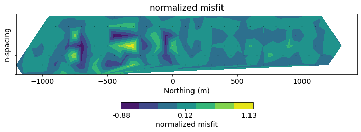
6.3 analyze the results - how did we get here?
def plot_beta(inversion_results, x="iteration", ax=None):
    """
    Plot the beta-value as a function of iteration
    """
    if ax is None:
        fig, ax = plt.subplots(1, 1)
    if x not in ["iteration", "beta"]:
        raise Exception("beta should be plotted as a function of iteration or beta")
    ax.plot(inversion_results[x], inversion_results["beta"], "-oC0", label="$\\beta$")
    ax.set_ylabel("$\\beta$")
    ax.legend(loc=2)
    return ax

def plot_misfit_and_regularization(inversion_results, x="iteration", ax=None):
    """
    Plot the data misfit and regularization as a function of iteration
    """
    if ax is None:
        fig, ax = plt.subplots(1, 1)

    if x not in ["iteration", "beta"]:
        raise Exception("misfit and regularization should be plotted as a function of iteration or beta")

    ax.plot(inversion_results[x], inversion_results["phi_d"], "-oC1", label="$\Phi_d$")
    ax.axhline(phi_d_star, linestyle="--", color="k", label="$\Phi_d^*$")
    ax.axhline(phi_d_star, linestyle="-.", color="k", label="$\chi\Phi_d^*$")
    ax.set_ylabel("$\Phi_d$")

    ax_phim = ax.twinx()
    ax_phim.plot(inversion_results[x], inversion_results["phi_m"], "-oC2", label="$\Phi_m$")
    ax_phim.set_ylabel("$\Phi_m$")
    ax.set_xlabel(x)

    ax.legend(loc=2)
    ax_phim.legend(loc=1)
    return ax

def plot_regularization_components(inversion_results, x="iteration", ax=None):
    """
    Plot the smallness and smoothness terms in the regularization as a function of iteration
    """
    if ax is None:
        fig, ax = plt.subplots(1, 1)

    if x not in ["iteration", "beta"]:
        raise Exception("regularization components should be plotted as a function of iteration or beta")

    ax.plot(inversion_results[x], inversion_results["phi_m_small"], "-oC3", label="$\\alpha_s\Phi_s$")
    ax.plot(inversion_results[x], inversion_results["phi_m_smooth_x"], "-oC4", label="$\\alpha_x\Phi_x$")
    ax.plot(inversion_results[x], inversion_results["phi_m_smooth_z"], "-oC5", label="$\\alpha_z\Phi_z$")
    ax.set_ylabel("$\Phi_m$")
    ax.set_xlabel(x)
    ax.legend(loc=2)
    return ax

def plot_tikhonov_curve(inversion_results, ax=None):
    """
    Plot the Tikhonov curve: Phi_d as a function of Phi_m
    """
    if ax is None:
        fig, ax = plt.subplots(1, 1)

    ax.plot(inversion_results["phi_m"], inversion_results["phi_d"], "-oC6", label="$\Phi_d$")
    ax.axhline(phi_d_star, linestyle="--", color="k", label="$\Phi_d^*$")
    ax.axhline(phi_d_star, linestyle="-.", color="k", label="$\chi\Phi_d^*$")
    ax.set_ylabel("$\Phi_d$")
    ax.set_xlabel(x)

    ax.set_xlabel("$\Phi_m$")
    ax.set_ylabel("$\Phi_d$")

    ax.legend(loc=1)
    return ax
fig, ax = plt.subplots(3, 1, figsize=(10, 8), sharex=True)
plot_beta(inversion_results, ax=ax[0])
plot_misfit_and_regularization(inversion_results, ax=ax[1])
plot_regularization_components(inversion_results, ax=ax[2])
ax[2].set_xlabel("iteration")Text(0.5, 0, 'iteration')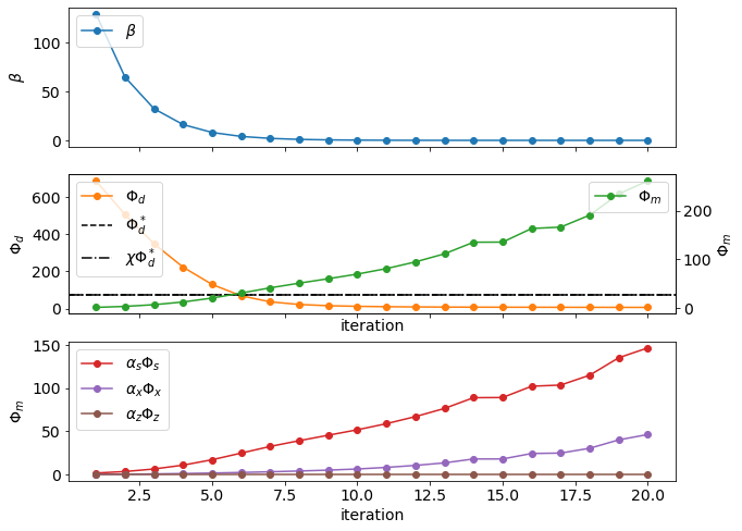
plot_tikhonov_curve(inversion_results)<AxesSubplot:xlabel='$\\Phi_m$', ylabel='$\\Phi_d$'>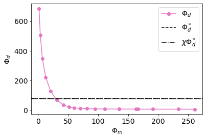
6.3 recovered model
def plot_model(
    model=model_recovered, ax=None, clim=np.exp(np.r_[np.min(model_true), np.max(model_true)]),
    colorbar=True, zlim=np.r_[-400, 0]
):
    """
    A plotting function for our recovered model
    """
    if ax is None:
        fig, ax = plt.subplots(1, 1)

    out = mesh.plotImage(
        mapping * model, pcolorOpts={'norm':LogNorm(), 'cmap':'Spectral'}, ax=ax,
        clim=clim
    )

    ax.set_xlim(core_domain_x)
    ax.set_ylim(zlim)
    ax.set_ylabel('Elevation (m)')
    ax.set_xlabel('Easting (m)')
    ax.set_aspect(1.5)  # some vertical exxageration

    if colorbar is True:
        cb = plt.colorbar(out[0], fraction=0.05, orientation='horizontal', ax=ax, pad=0.25)
        cb.set_label("Resistivity ($\Omega$m)")

    return ax
6.4 Explore the results as a function of iteration
def plot_results_at_iteration(iteration=0):
    """
    A function to plot inversion results as a function of iteration
    """
    fig = plt.figure(figsize=(12, 8))
    spec = gridspec.GridSpec(ncols=6, nrows=2, figure=fig)

    ax_tikhonov = fig.add_subplot(spec[:, :2])
    ax_misfit = fig.add_subplot(spec[0, 2:])
    ax_model = fig.add_subplot(spec[1, 2:])

    plot_tikhonov_curve(inversion_results, ax=ax_tikhonov)
    ax_tikhonov.plot(
        inversion_results["phi_m"][iteration], inversion_results["phi_d"][iteration],
        'ks', ms=10
    )
    ax_tikhonov.set_title(f"iteration {iteration}")

    plot_normalized_misfit(iteration=iteration, ax=ax_misfit)

    plot_model(inversion_results["model"][iteration], ax=ax_model, )
    # make the tikhonov plot square
    ax_tikhonov.set_aspect(1./ax_tikhonov.get_data_ratio())

    plt.tight_layout()
inversion_results_app = ipywidgets.interact(
plot_results_at_iteration,
iteration = ipywidgets.IntSlider(min=0, max=inversion_results["iteration"][-1]-1, value=0)
)
inversion_results_app6.5 Compare with the True model
fig, ax = plt.subplots(2, 1, figsize=(10, 8))
clim = np.exp(np.r_[model_true.min(), model_true.max()])
plot_model(model_recovered, clim=clim,  ax=ax[0])
plot_model(model_true, clim=clim,  ax=ax[1])
<AxesSubplot:xlabel='Easting (m)', ylabel='Elevation (m)'>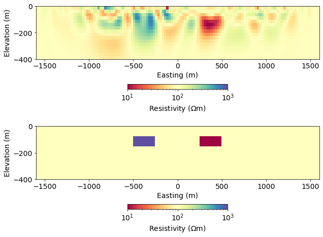
Homework ✏️
What happens if you introduce a layer above the blocks?
- Define a layer from z=-50 to z=-100.
- Start with a resistive layer.
- How does this change our ability to resolve the blocks?
- Now try with a conductive layer.
- Get creative! Build a model that interests you.
Send us your images and discussion on slack!