Forward simulations
In this notebook, we use a synthetic example to explore aspects of numerical modelling, including mesh design, as well as exploring aspects of the fundamental physics, including viewing the currents, charges and potentials from conductive and resistive targets.
Step 0: Imports and load survey info
These initial steps are the same as in the previous notebook.
# core python
import numpy as np
import matplotlib.pyplot as plt
from matplotlib.colors import LogNorm, SymLogNorm, Normalize
import ipywidgets

# tools in the simPEG Ecosystem
import discretize  # for creating computational meshes

# linear solvers
try:
    from pymatsolver import Pardiso as Solver  # this is a fast linear solver
except ImportError:
    from SimPEG import SolverLU as Solver  # this will be slower

# SimPEG inversion machinery
from SimPEG import Data, maps

# DC resistivity and IP modules
from SimPEG.electromagnetics import resistivity as dc
# set the font size in the plots
from matplotlib import rcParams
rcParams["font.size"] = 14Step 1: Load DC survey
As in the first notebook, we load up the survey geometry from our data file and create a SimPEG survey object.
line = "46800E"

dc_data_file = f"./century/{line}/{line[:-1]}POT.OBS"
def read_dcip_data(filename, verbose=True):
"""
Read in a .OBS file from the Century data set into a python dictionary.
The format is the old UBC-GIF DCIP format.
Parameters
----------
filename : str
Path to the file to be parsed
verbose: bool
Print some things?
Returns
-------
dict
A dictionary with the locations of
- a_locations: the positive source electrode locations (numpy array)
- b_locations: the negative source electrode locations (numpy array)
- m_locations: the receiver locations (list of numpy arrays)
- n_locations: the receiver locations (list of numpy arrays)
- n_locations: the receiver locations (list of numpy arrays)
- observed_data: observed data (list of numpy arrays)
- standard_deviations: assigned standard deviations (list of numpy arrays)
- n_sources: number of sources (int)
"""
# create an empty source_list
source_list = []
# read in the text file as a numpy array of strings (each row is an entry)
contents = np.genfromtxt(filename, delimiter=' \n', dtype=np.str)
# the second line has the number of sources, current, and data type (voltages if 1)
n_sources = int(contents[1].split()[0])
if verbose is True:
print(f"number of sources: {n_sources}")
# initialize storage for the electrode locations and data
a_locations = np.zeros(n_sources)
b_locations = np.zeros(n_sources)
m_locations = []
n_locations = []
observed_data = []
standard_deviations = []
# index to track where we have read in content
content_index = 1
# loop over sources
for i in range(n_sources):
# start by reading in the source info
content_index = content_index + 1 # read the next line
a_location, b_location, nrx = contents[content_index].split() # this is a string
# convert the strings to a float for locations and an int for the number of receivers
a_locations[i] = float(a_location)
b_locations[i] = float(b_location)
nrx = int(nrx)
if verbose is True:
print(f"Source {i}: A-loc: {a_location}, B-loc: {b_location}, N receivers: {nrx}")
# initialize space for receiver locations, observed data associated with this source
m_locations_i, n_locations_i = np.zeros(nrx), np.zeros(nrx)
observed_data_i, standard_deviations_i = np.zeros(nrx), np.zeros(nrx)
# read in the receiver info
for j in range(nrx):
content_index = content_index + 1 # read the next line
m_location, n_location, datum, std = contents[content_index].split()
# convert the locations and data to floats, and store them
m_locations_i[j] = float(m_location)
n_locations_i[j] = float(n_location)
observed_data_i[j] = float(datum)
standard_deviations_i[j] = float(std)
# append the receiver info to the lists
m_locations.append(m_locations_i)
n_locations.append(n_locations_i)
observed_data.append(observed_data_i)
standard_deviations.append(standard_deviations_i)
return {
"a_locations": a_locations,
"b_locations": b_locations,
"m_locations": m_locations,
"n_locations": n_locations,
"observed_data": observed_data,
"standard_deviations": standard_deviations,
"n_sources": n_sources,
}dc_data_dict = read_dcip_data(dc_data_file, verbose=False)# initialize an empty list for each
source_list = []
# center the survey and work in local coordinates
x_local = 0.5*(np.min(dc_data_dict["a_locations"]) + np.max(np.hstack(dc_data_dict["n_locations"])))
for i in range(dc_data_dict["n_sources"]):
# receiver electrode locations in 2D
m_locs = np.vstack([
dc_data_dict["m_locations"][i] - x_local,
np.zeros_like(dc_data_dict["m_locations"][i])
]).T
n_locs = np.vstack([
dc_data_dict["n_locations"][i] - x_local,
np.zeros_like(dc_data_dict["n_locations"][i])
]).T
# construct the receiver object
receivers = dc.receivers.Dipole(locations_m=m_locs, locations_n=n_locs, storeProjections=False)
# construct the source
source = dc.sources.Dipole(
location_a=np.r_[dc_data_dict["a_locations"][i] - x_local, 0.],
location_b=np.r_[dc_data_dict["b_locations"][i] - x_local, 0.],
receiver_list=[receivers]
)
# append the new source to the source list
source_list.append(source)survey = dc.Survey(source_list=source_list)Exploration 1: how does mesh design impact accuracy?
In what follows, we will build up several functions that allow us to design a mesh and compare the simulated apparent resistivity and the true half-space resistivity in order to assess the mesh design.
def build_mesh(
    survey=survey,
    n_cells_per_spacing_x=4,
    n_cells_per_spacing_z=4,
    n_core_extra_x=4,
    n_core_extra_z=4,
    core_domain_z_ratio=1/3.,
    padding_factor=1.3,
    n_pad_x=10,
    n_pad_z=10,
):
    """
    A function for designing a Tensor Mesh based on DC survey parameters

    Parameters
    ----------

    survey: dc.Survey
        A DC (or IP) survey object

    n_cells_per_spacing_[x, z]: int
        Number of [x, z]-cells per the minimum electrode spacing

    n_core_extra_[x, z]: int
        Number of extra cells with the same size as the core domain beyond the survey extent

    core_domain_z_ratio: float
        Factor that multiplies the maximum AB, MN separation to define the core mesh extent

    padding_factor: float
        Factor by which we expand the mesh cells in the padding region

    n_pad_[x, z]: int
        Number of padding cells in the x, z directions
    """
    min_electrode_spacing = np.min(np.abs(survey.locations_a[:, 0] - survey.locations_b[:, 0]))

    dx = min_electrode_spacing / n_cells_per_spacing_x
    dz = min_electrode_spacing / n_cells_per_spacing_z

    # define the x core domain
    core_domain_x = np.r_[
        survey.electrode_locations[:, 0].min(),
        survey.electrode_locations[:, 0].max()
    ]

    # find the y core domain
    # find the maximum spacing between source, receiver midpoints
    mid_ab = (survey.locations_a + survey.locations_b)/2
    mid_mn = (survey.locations_m + survey.locations_n)/2
    separation_ab_mn = np.abs(mid_ab - mid_mn)
    max_separation = separation_ab_mn.max()
    core_domain_z = np.r_[-core_domain_z_ratio * max_separation, 0.]

    # add extra cells beyond the core domain
    n_core_x = np.ceil(np.diff(core_domain_x)/dx) + n_core_extra_x*2  # on each side
    n_core_z = np.ceil(np.diff(core_domain_z)/dz) + n_core_extra_z  # just below

    # define the tensors in each dimension
    hx = [(dx, n_pad_x, -padding_factor), (dx, n_core_x), (dx, n_pad_x, padding_factor)]
    hz = [(dz, n_pad_z, -padding_factor), (dz, n_core_z)]

    mesh = discretize.TensorMesh([hx, hz], x0="CN")

    return mesh, core_domain_x, core_domain_z
mesh, core_domain_x, core_domain_z = build_mesh(survey)
mesh.plotGrid()<AxesSubplot:xlabel='x1', ylabel='x2'>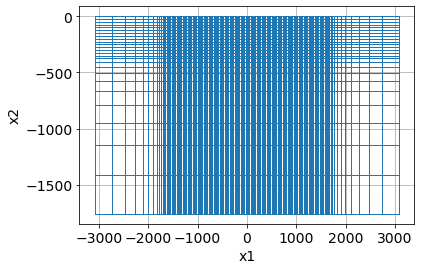
meshdef forward_simulation_halfspace(mesh, survey=survey, resistivity=100, nky=11):
"""
A function that returns predicted data given a mesh, survey,
resistivity value and number of filters for the 2.5 DC simulation.
"""
# clear the stored source values if they were previously computed
for src in survey.source_list:
src._q = None
rho = resistivity * np.ones(mesh.nC)
simulation_dc = dc.Simulation2DNodal(
mesh, rhoMap=maps.IdentityMap(mesh), solver=Solver,
survey=survey, nky=nky
)
dpred = simulation_dc.make_synthetic_data(rho)
# clear the stored source values if they were previously computed
for src in survey.source_list:
src._q = None
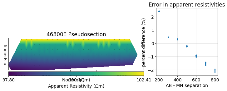
return dpreddef plot_apparent_resistivities(dpred, halfspace_resistivity):
"""
Plot the apparent resistivity given a SimPEG data object
and the true halfspace resistivity.
"""
# plot psuedosection
fig = plt.figure(constrained_layout=True, figsize=(12, 4))
gs = fig.add_gridspec(ncols=3, nrows=1)
ax0 = fig.add_subplot(gs[:2])
ax1 = fig.add_subplot(gs[2])
# plot the pseudosection
dc.utils.plot_pseudosection(
dpred, data_type="apparent resistivity", # clim=clim,
plot_type="pcolor", data_location=True, ax=ax0,
)
ax0.set_aspect(2) # some vertical exxageration
ax0.set_title(f"{line} Pseudosection")
ax0.set_xlabel("Northing (m)")
ax0.set_yticks([])
# plot the errors in apparent resistivity relative to separation
mid_ab = (survey.locations_a + survey.locations_b)/2
mid_mn = (survey.locations_m + survey.locations_n)/2
separation_ab_mn = np.abs(mid_ab - mid_mn)
apparent_resistivity = dc.utils.apparent_resistivity(dpred)
percent_error = (apparent_resistivity - halfspace_resistivity)/halfspace_resistivity*100
ax1.plot(separation_ab_mn[:, 0], percent_error, '.', alpha=0.4)
ax1.set_xlabel("AB - MN separation")
ax1.set_ylabel("percent difference (%)")
ax1.set_title("Error in apparent resistivities")
ax1.grid(alpha=0.3)
halfspace_resistivity = 100
dpred = forward_simulation_halfspace(mesh, resistivity=halfspace_resistivity)
plot_apparent_resistivities(dpred, halfspace_resistivity)
/srv/conda/envs/notebook/lib/python3.7/site-packages/SimPEG/electromagnetics/static/utils/static_utils.py:468: MatplotlibDeprecationWarning: shading='flat' when X and Y have the same dimensions as C is deprecated since 3.3. Either specify the corners of the quadrilaterals with X and Y, or pass shading='auto', 'nearest' or 'gouraud', or set rcParams['pcolor.shading']. This will become an error two minor releases later.
**pcolor_opts,
/srv/conda/envs/notebook/lib/python3.7/site-packages/SimPEG/electromagnetics/static/utils/static_utils.py:523: UserWarning: FixedFormatter should only be used together with FixedLocator
ax.set_yticklabels(-ticks / spacing)
/srv/conda/envs/notebook/lib/python3.7/site-packages/IPython/core/pylabtools.py:132: UserWarning: constrained_layout not applied. At least one axes collapsed to zero width or height.
fig.canvas.print_figure(bytes_io, **kw)
def mesh_design_simulator(
    survey=survey,
    n_cells_per_spacing_x=4,
    n_cells_per_spacing_z=4,
    n_core_extra_x=4,
    n_core_extra_z=4,
    core_domain_z_ratio=1/3.,
    padding_factor=1.3,
    n_pad_x=10,
    n_pad_z=10,
    log10_halfspace_resistivity=2,
    nky=11,
):
    """
    A function that brings together mesh design and forward simulation so
    that we can interactively explore factors of mesh design that influence
    the accuracy of our simulation.
    """

    # set up mesh
    mesh, core_domain_x, core_domain_z = build_mesh(
        survey=survey,
        n_cells_per_spacing_x=n_cells_per_spacing_x,
        n_cells_per_spacing_z=n_cells_per_spacing_z,
        n_core_extra_x=n_core_extra_x,
        n_core_extra_z=n_core_extra_z,
        core_domain_z_ratio=core_domain_z_ratio,
        padding_factor=padding_factor,
        n_pad_x=n_pad_x,
        n_pad_z=n_pad_z,
    )

    # convert the log10 resistivity to true resistivity on the mesh
    halfspace_resistivity = 10**log10_halfspace_resistivity

    # compute predicted data
    dpred = forward_simulation_halfspace(mesh, resistivity=halfspace_resistivity, nky=nky)

    # plot those apparent resistivities
    plot_apparent_resistivities(dpred, halfspace_resistivity)
mesh_design_app = ipywidgets.interactive(
mesh_design_simulator,
survey=ipywidgets.fixed(survey),
n_cells_per_spacing_x=ipywidgets.IntSlider(
description="nCx p. 100m", min=1, max=10, value=4, continuous_update=False
),
n_cells_per_spacing_z=ipywidgets.IntSlider(
description="nCz p. 100m", min=1, max=10, value=4, continuous_update=False
),
n_core_extra_x=ipywidgets.IntSlider(
description="ncore x +", min=0, max=10, value=4, continuous_update=False
),
n_core_extra_z=ipywidgets.IntSlider(
description="ncore z +", min=0, max=10, value=4, continuous_update=False
),
core_domain_z_ratio=ipywidgets.FloatSlider(
description="Dz*maxABMN", min=0.1, max=1, value=0.3, continuous_update=False
),
padding_factor=ipywidgets.FloatSlider(
description="pad factor", min=1, max=5, value=1.3, continuous_update=False
),
n_pad_x=ipywidgets.IntSlider(
min=1, max=20, value=10, continuous_update=False
),
n_pad_z=ipywidgets.IntSlider(
min=1, max=20, value=10, continuous_update=False
),
log10_halfspace_resistivity=ipywidgets.FloatSlider(
description="$log_{10}\\rho$", min=-1, max=7, value=2, continuous_update=False
),
nky=ipywidgets.IntSlider(
min=1, max=20, value=11, continuous_update=False
)
)Questions: Mesh design
- Which offsets are most affected if we change the number of cells per electrode spacing (the sliders labeled:
nCx p. 100m,nCz p. 100m)? - What about if we change the padding?
- What happens if we reduce the number of padding cells but increase the padding factor?
mesh_design_appExploration 2: the physics
Forward simulations can be a powerful tool for building up understanding and intuition for a given geophysical experiment. In SimPEG, we expose the ability to access the fields and fluxes computed in a simulation through the fields object that contains the solution to the PDE everywhere on the mesh. This is an intermediate step when computing predicted data, and in an inversion, we would typically not store them.
Here, we build up a simple synthetic model that includes 2 blocks, one resistive and one conductive, in a halfspace. We will visualize the currents, charges and electric fields.
Define the model
# define the resistivities
rho_background = 100
rho_resistive_block = 1000
rho_conductive_block = 10

# define the geometry of each block
xlim_resistive_block = np.r_[-500, -250]
zlim_resistive_block = np.r_[-250, -100]

xlim_conductive_block = np.r_[250, 500]
zlim_conductive_block = np.r_[-250, -100]
Put the model on the mesh
For the simulation, we define physical properties on the cell centers of the mesh. In discretize, once we have created a mesh, the cell-centered grid is accessible through the gridCC property. Columns correspond to each of the dimensions, so the shape of gridCC is (number of cells, number of dimensions).
rho = rho_background * np.ones(mesh.nC)

# resistive block
inds_resistive_block = (
    (mesh.gridCC[:, 0] >= xlim_resistive_block.min()) & (mesh.gridCC[:, 0] <= xlim_resistive_block.max()) &
    (mesh.gridCC[:, 1] >= zlim_resistive_block.min()) & (mesh.gridCC[:, 1] <= zlim_resistive_block.max())
)

rho[inds_resistive_block] = rho_resistive_block

# conductive block
inds_conductive_block = (
    (mesh.gridCC[:, 0] >= xlim_conductive_block.min()) & (mesh.gridCC[:, 0] <= xlim_conductive_block.max()) &
    (mesh.gridCC[:, 1] >= zlim_conductive_block.min()) & (mesh.gridCC[:, 1] <= zlim_conductive_block.max())
)

rho[inds_conductive_block] = rho_conductive_block
fig, ax = plt.subplots(1, 1, figsize=(12, 4))
out = mesh.plotImage(np.log10(rho), ax=ax)
plt.colorbar(out[0], ax=ax, label="log$_{10} \\rho$")
ax.set_xlim(core_domain_x)
ax.set_ylim(core_domain_z + np.r_[-100, 0])
ax.set_aspect(1.5)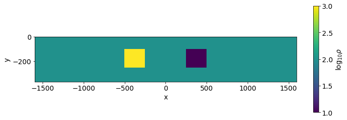
Set up the forward simulation
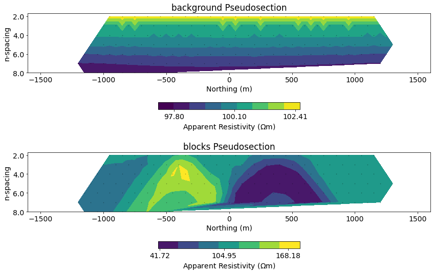
As in the previous notebook, we set up a forward simulation. In this case, we use an IdentityMap for the mapping, so we directly provide resistivity values to the forward simulation. In order to be able to explore the impact of both the blocks on our measured data, we will run simulations for both the halfspace background and for the model containing two blocks.
mapping = maps.IdentityMap(mesh)

# Generate 2.5D DC problem
simulation_dc = dc.Simulation2DNodal(
    mesh, rhoMap=mapping, solver=Solver, survey=survey
)
%%time
# run the forward simulation over the half-space
model_background = rho_background * np.ones(mesh.nC)
fields_background = simulation_dc.fields(model_background)
synthetic_data_background = simulation_dc.make_synthetic_data(model_background, f=fields_background)CPU times: user 711 ms, sys: 67.1 ms, total: 778 ms
Wall time: 1.25 s
%%time

# run the forward simulation over the full model
fields = simulation_dc.fields(rho)
synthetic_data = simulation_dc.make_synthetic_data(rho, f=fields)
CPU times: user 610 ms, sys: 49.2 ms, total: 659 ms
Wall time: 1.01 s
# plot both pseudosections
fig, ax = plt.subplots(2, 1, figsize=(12, 8))

for a, plot_data, title in zip(
    ax, [synthetic_data_background, synthetic_data], ["background", "blocks"]
):

    # plot a psuedosection of the data
    dc.utils.plot_pseudosection(
        plot_data, data_type="apparent resistivity",
        plot_type="contourf", data_location=True, ax=a,
        cbar_opts={"pad":0.25}
    )
    a.set_title(f"{title} Pseudosection")
    a.set_xlim(core_domain_x)
    a.set_aspect(1.5)  # some vertical exxageration
    a.set_xlabel("Northing (m)")

plt.tight_layout()
/srv/conda/envs/notebook/lib/python3.7/site-packages/SimPEG/electromagnetics/static/utils/static_utils.py:523: UserWarning: FixedFormatter should only be used together with FixedLocator
  ax.set_yticklabels(-ticks / spacing)
/srv/conda/envs/notebook/lib/python3.7/site-packages/SimPEG/electromagnetics/static/utils/static_utils.py:523: UserWarning: FixedFormatter should only be used together with FixedLocator
  ax.set_yticklabels(-ticks / spacing)
Define a plotting function to visualize aspects of the physics
In a Nodal discretization for the DC problem:
- physical properties are at cell centers (CC)
- charge density is at cell centers (CC)
- electric potentials (
phi) are at cell nodes (N) - electric fields (
e) are on cell edges (E) - current density (
j) is on cell edges (E)
For plotting purposes, we will average to cell centers. To average the scalar phi values from nodes to cell centers, we use the aveN2CC operator. To average vector quantities (e, j) to cell centers, we use the aveE2CCV operator (V for vector).
def plot_physics(field="phi", primsec="total", scale="linear", source_ind=0):
"""
A function for plotting aspects of the forward simulation
"""
fig, ax = plt.subplots(2, 1, figsize=(12, 8))
pcolor_opts = {}
view = "real"
vType = "CC"
source = survey.source_list[source_ind]
# plotting resistivities
if field == "model":
plotme = rho
if primsec == "primary":
plotme = model_background
elif primsec == "secondary":
plotme = plotme - model_background
if scale.lower() == "log":
pcolor_opts["norm"] = LogNorm()
# plotting the physics
else:
if primsec in ["total", "secondary"]:
plotme = fields[source, field]
if primsec == "secondary":
plotme -= fields_background[source, field]
else:
plotme = fields_background[source, field]
# average the potentials to cell centers from Nodes
if field == "phi":
plotme = mesh.aveN2CC * plotme
# average the fields to cell centers
elif field in ["j", "e"]:
view = "vec"
vType = "CCv"
plotme = mesh.aveE2CCV * plotme
if scale.lower() == "log":
pcolor_opts["norm"] = LogNorm()
# set an intuitive colorbar for charges
elif field == "charge_density":
pcolor_opts["cmap"] = "RdBu_r"
# set a symmetric colorbar
if field in ["phi", "charge_density"]:
max_abs = np.abs(plotme).max()
if scale.lower() == "linear":
pcolor_opts["norm"] = Normalize(vmin=-max_abs, vmax=max_abs)
if scale.lower() == "log":
pcolor_opts["norm"] = SymLogNorm(
linthresh=max_abs * 1e-3, vmin=-max_abs, vmax=max_abs
)
# plot the physics
out = mesh.plotImage(
plotme, view=view, vType=vType, pcolorOpts=pcolor_opts, ax=ax[0],
range_x=core_domain_x, range_y=core_domain_z,
)
ax[0].plot([source.location_a[0], source.location_b[0]], np.r_[5, 5], "vC3", ms=8)
ax[0].set_ylim(core_domain_z + np.r_[-100, 0])
plt.colorbar(out[0], ax=ax[0], label=field, fraction=0.1, orientation="horizontal", pad=0.25)
# plot a psuedosection of the data
dc.utils.plot_pseudosection(
synthetic_data, data_type="apparent resistivity", # clim=clim,
plot_type="contourf", data_location=True, ax=ax[1],
cbar_opts={"pad":0.25}
)
ax[1].set_title(f"{line} Pseudosection")
for a in ax:
a.set_xlim(core_domain_x)
a.set_aspect(1.5) # some vertical exxageration
a.set_xlabel("Northing (m)")
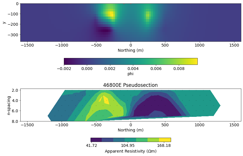
plt.tight_layout()plot_physics(field="phi", primsec="secondary", source_ind=15)/srv/conda/envs/notebook/lib/python3.7/site-packages/discretize/View.py:481: MatplotlibDeprecationWarning: Passing parameters norm and vmin/vmax simultaneously is deprecated since 3.3 and will become an error two minor releases later. Please pass vmin/vmax directly to the norm when creating it.
out += (ax.pcolormesh(self.vectorNx, self.vectorNy, v.T, vmin=clim[0], vmax=clim[1], **pcolor_opts), )
/srv/conda/envs/notebook/lib/python3.7/site-packages/SimPEG/electromagnetics/static/utils/static_utils.py:523: UserWarning: FixedFormatter should only be used together with FixedLocator
ax.set_yticklabels(-ticks / spacing)
dc_physics_app = ipywidgets.interactive(
    plot_physics,
    field=ipywidgets.ToggleButtons(options=["model", "j", "e", "charge_density", "phi"], value="model"),
    primsec=ipywidgets.ToggleButtons(options=["total", "primary", "secondary"], value="total"),
    scale=ipywidgets.ToggleButtons(options=["linear", "log"]),
    source_ind=ipywidgets.IntSlider(min=0, max=len(survey.source_list)-1, value=15),
)
Questions: Physics of DC
- Where do currents preferentially flow?
- Where do charges build up? How does that depend on the location of the source?
dc_physics_appHomework ✏️
What happens if you introduce a layer above the blocks?
- Define a layer from z=-50 to z=-100.
- Start with a resistive layer.
- How does that change the currents? charges?
- Do we still see the evidence of the blocks in the data (Hint: compare those data with a model that contains the layer but not the block)
- Now try with a conductive layer.
Send us your images and discussion on slack!