Inversion of DC & IP data at the Century Deposit
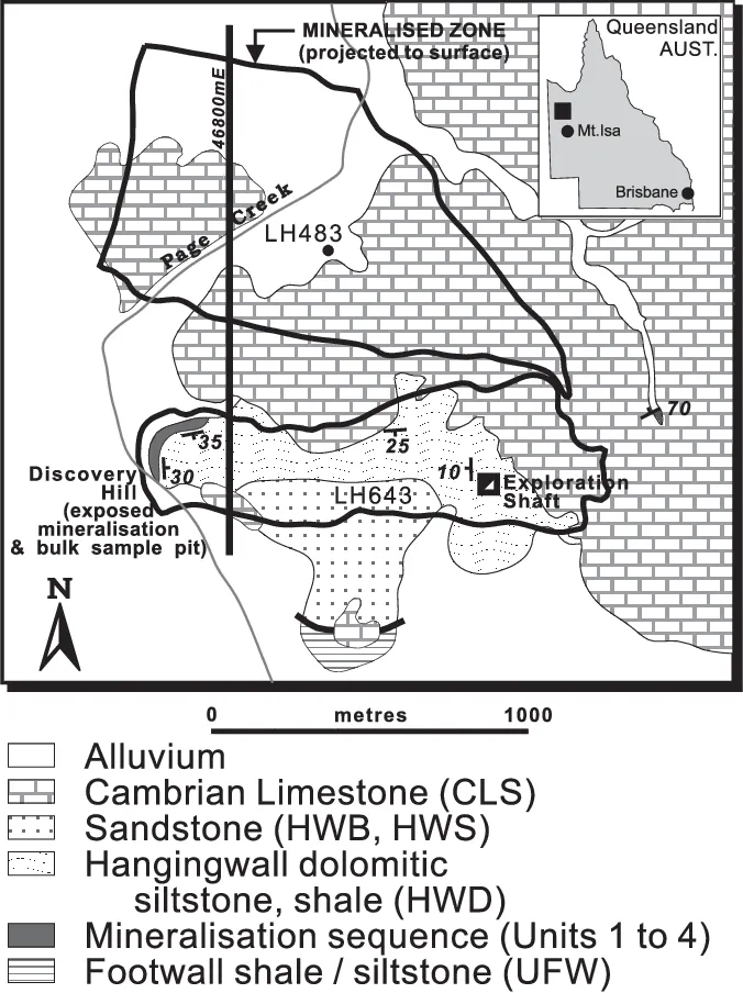
The Century Deposit is a Zinc-lead-silver deposit is located 250 km to the NNW of the Mt Isa region in Queensland Australia (Location: 18° 43' 15"S, 138° 35' 54"E).
References
For background on DC Resistivity Surveys, see GPG: DC Resistivity
In this notebook, we are going to invert the data and see if we can replicate the results presented in Mutton, 2000. Specifically, we will work with data collected along the line 46800mE.
Motivation: replicate inversion results from 20 years ago!

The image below shows the Induced Polarization inversion result generated using the UBC 2D DCIP inversion code that was published in Mutton, 2000.
Can we replicate it with SimPEG?
(and update the colorbar 😉)

Step 0: Import Dependencies
Here are links to the documentation for each of the packages we rely on for this tutorial.
Core Python / Jupyter
- numpy: arrays
- matplotlib: plotting
- ipywidgets: interactive widgets in jupyter
SimPEG ecosystem
- discretize: meshes and differential operators
- pymatsolver: wrappers on linear solvers
- SimPEG: Simulation and Parameter Estimation in Geophysics
import warnings
warnings.filterwarnings("ignore")
# core python
import numpy as np
import matplotlib.pyplot as plt
from matplotlib.colors import LogNorm
import ipywidgets
import os
# tools in the simPEG Ecosystem
import discretize # for creating computational meshes
# linear solvers
try:
from pymatsolver import Pardiso as Solver # this is a fast linear solver
except ImportError:
from SimPEG import SolverLU as Solver # this will be slower
# SimPEG inversion machinery
from SimPEG import (
Data, maps,
data_misfit, regularization, optimization, inverse_problem,
inversion, directives
)
# DC resistivity and IP modules
from SimPEG.electromagnetics import resistivity as dc
from SimPEG.electromagnetics import induced_polarization as ip# set the font size in the plots
from matplotlib import rcParams
rcParams["font.size"] = 14Step 1: Load the data
What are our data?
The survey collected at the Century Deposit uses a dipole-dipole geometry with:
- Current Electrodes (A, B): we refer to the source electrodes as "A" for the positive electrode and "B" for the negative electrode.
- Potential Electrodes (M, N): we refer to the positive potential electrode as "M" and the negative as "N".
A datum is the potential difference between the M and N electrodes.


The data are stored in the century directory. Here, we take a look at what is in that directory. Each folder contains data associated with the named line.
os.listdir('century')['46800E',
'.DS_Store',
'46200E',
'47200E',
'geologic_section.csv',
'Data_in_3D_format',
'47700E',
'27750N',
'gmt',
'47000E']We will focus on the 46800E line. In that directory, there are several files. The .OBS files are the observed data. The other files are previous inversion results from the UBC inversion. For the two .OBS files: POT refers to "Potentials" - these are our DC data and IP refers to "Induced Polarization". We will start by working with the DC resistivity data and so will load up that file first.
line = "46800E"
print(os.listdir(os.path.join('century',line)))

dc_data_file = f"./century/{line}/{line[:-1]}POT.OBS"
['DCMODA.LOG', 'DCMODA.PRE', '.DS_Store', '46800POT.OBS', 'IPMODA.OUT', '468MESH.DAT', 'IPMODA.CHG', 'DCMODA.OUT', 'IPMODA.PRE', '46800IP.OBS', 'DCMODA.CON', 'IPMODA.LOG']
These file formats are an older version of the UBC DC format and are very similar to the current UBC DC IP Surface Format
Comment line: description of data
   n_sources dipole(1) dipole(1)
     A_location  B_location   n_receivers
   M_location  N_location  measured_potential  standard_deviation
   M_location  N_location  measured_potential  standard_deviation
     A_location  B_location   n_receivers
   M_location  N_location  measured_potential  standard_deviation
   M_location  N_location  measured_potential  standard_deviation
   ....
with open(dc_data_file) as f:
print(f.read())AVG-GDAT 1.22: CENTURY Converted by RES2POT to conductivitie
27 1 1
26000.000000 26100.000000 2
26700.0 26800.0 -.00127 .00006
26800.0 26900.0 -.00080 .00004
26100.000000 26200.000000 3
26700.0 26800.0 -.00164 .00008
26800.0 26900.0 -.00099 .00005
26900.0 27000.0 -.00063 .00003
26200.000000 26300.000000 4
26700.0 26800.0 -.00252 .00013
26800.0 26900.0 -.00146 .00007
26900.0 27000.0 -.00088 .00004
27000.0 27100.0 -.00125 .00006
26300.000000 26400.000000 5
26700.0 26800.0 -.00504 .00025
26800.0 26900.0 -.00260 .00013
26900.0 27000.0 -.00147 .00007
27000.0 27100.0 -.00195 .00010
27100.0 27200.0 -.00103 .00005
26400.000000 26500.000000 6
26700.0 26800.0 -.01048 .00052
26800.0 26900.0 -.00472 .00024
26900.0 27000.0 -.00249 .00012
27000.0 27100.0 -.00300 .00015
27100.0 27200.0 -.00146 .00007
27200.0 27300.0 -.00122 .00006
26500.000000 26600.000000 7
26700.0 26800.0 -.02069 .00103
26800.0 26900.0 -.00690 .00034
26900.0 27000.0 -.00313 .00016
27000.0 27100.0 -.00342 .00017
27100.0 27200.0 -.00152 .00008
27200.0 27300.0 -.00121 .00006
27300.0 27400.0 -.00074 .00004
26600.000000 26700.000000 7
26800.0 26900.0 -.03448 .00172
26900.0 27000.0 -.01074 .00054
27000.0 27100.0 -.00934 .00047
27100.0 27200.0 -.00347 .00017
27200.0 27300.0 -.00244 .00012
27300.0 27400.0 -.00142 .00007
27400.0 27500.0 -.00075 .00004
26700.000000 26800.000000 6
26900.0 27000.0 -.05464 .00273
27000.0 27100.0 -.02931 .00147
27100.0 27200.0 -.00769 .00038
27200.0 27300.0 -.00446 .00022
27300.0 27400.0 -.00238 .00012
27400.0 27500.0 -.00112 .00006
26800.000000 26900.000000 6
27000.0 27100.0 -.09178 .00459
27100.0 27200.0 -.01432 .00072
27200.0 27300.0 -.00684 .00034
27300.0 27400.0 -.00334 .00017
27400.0 27500.0 -.00156 .00008
27500.0 27600.0 -.00057 .00003
26900.000000 27000.000000 6
27100.0 27200.0 -.03661 .00183
27200.0 27300.0 -.01141 .00057
27300.0 27400.0 -.00515 .00026
27400.0 27500.0 -.00218 .00011
27500.0 27600.0 -.00071 .00004
27600.0 27700.0 -.00044 .00002
27000.000000 27100.000000 6
27200.0 27300.0 -.06844 .00342
27300.0 27400.0 -.02600 .00130
27400.0 27500.0 -.00971 .00049
27500.0 27600.0 -.00257 .00013
27600.0 27700.0 -.00139 .00007
27700.0 27800.0 -.00094 .00005
27100.000000 27200.000000 6
27300.0 27400.0 -.04881 .00244
27400.0 27500.0 -.01658 .00083
27500.0 27600.0 -.00361 .00018
27600.0 27700.0 -.00170 .00008
27700.0 27800.0 -.00103 .00005
27800.0 27900.0 -.00077 .00004
27200.000000 27300.000000 6
27400.0 27500.0 -.23608 .01180
27500.0 27600.0 -.02056 .00103
27600.0 27700.0 -.00520 .00026
27700.0 27800.0 -.00265 .00013
27800.0 27900.0 -.00180 .00009
27900.0 28000.0 -.00147 .00007
27300.000000 27400.000000 6
27500.0 27600.0 -.14165 .00708
27600.0 27700.0 -.01565 .00078
27700.0 27800.0 -.00504 .00025
27800.0 27900.0 -.00300 .00015
27900.0 28000.0 -.00206 .00010
28000.0 28100.0 -.00199 .00010
27400.000000 27500.000000 6
27600.0 27700.0 -.10451 .00523
27700.0 27800.0 -.01194 .00060
27800.0 27900.0 -.00504 .00025
27900.0 28000.0 -.00302 .00015
28000.0 28100.0 -.00265 .00013
28100.0 28200.0 -.00137 .00007
27500.000000 27600.000000 6
27700.0 27800.0 -.06472 .00324
27800.0 27900.0 -.01459 .00073
27900.0 28000.0 -.00541 .00027
28000.0 28100.0 -.00398 .00020
28100.0 28200.0 -.00179 .00009
28200.0 28300.0 -.00134 .00007
27600.000000 27700.000000 6
27800.0 27900.0 -.10186 .00509
27900.0 28000.0 -.01857 .00093
28000.0 28100.0 -.00971 .00049
28100.0 28200.0 -.00334 .00017
28200.0 28300.0 -.00211 .00011
28300.0 28400.0 -.00131 .00007
27700.000000 27800.000000 6
27900.0 28000.0 -.06525 .00326
28000.0 28100.0 -.02348 .00117
28100.0 28200.0 -.00642 .00032
28200.0 28300.0 -.00363 .00018
28300.0 28400.0 -.00206 .00010
28400.0 28500.0 -.00115 .00006
27800.000000 27900.000000 6
28000.0 28100.0 -.10133 .00507
28100.0 28200.0 -.01592 .00080
28200.0 28300.0 -.00711 .00036
28300.0 28400.0 -.00350 .00018
28400.0 28500.0 -.00177 .00009
28500.0 28600.0 -.00089 .00004
27900.000000 28000.000000 6
28100.0 28200.0 -.09178 .00459
28200.0 28300.0 -.02666 .00133
28300.0 28400.0 -.01019 .00051
28400.0 28500.0 -.00430 .00021
28500.0 28600.0 -.00194 .00010
28600.0 28700.0 -.00198 .00010
28000.000000 28100.000000 6
28200.0 28300.0 -.17931 .00897
28300.0 28400.0 -.04748 .00237
28400.0 28500.0 -.01533 .00077
28500.0 28600.0 -.00602 .00030
28600.0 28700.0 -.00561 .00028
28700.0 28800.0 -.00237 .00012
28100.000000 28200.000000 6
28300.0 28400.0 -.14271 .00714
28400.0 28500.0 -.03316 .00166
28500.0 28600.0 -.01151 .00058
28600.0 28700.0 -.00997 .00050
28700.0 28800.0 -.00387 .00019
28800.0 28900.0 -.00234 .00012
28200.000000 28300.000000 6
28400.0 28500.0 -.09072 .00454
28500.0 28600.0 -.02520 .00126
28600.0 28700.0 -.02064 .00103
28700.0 28800.0 -.00743 .00037
28800.0 28900.0 -.00432 .00022
28900.0 29000.0 -.00382 .00019
28300.000000 28400.000000 6
28500.0 28600.0 -.06950 .00347
28600.0 28700.0 -.04417 .00221
28700.0 28800.0 -.01416 .00071
28800.0 28900.0 -.00775 .00039
28900.0 29000.0 -.00668 .00033
29000.0 29100.0 -.00417 .00021
28400.000000 28500.000000 6
28600.0 28700.0 -.09125 .00456
28700.0 28800.0 -.02268 .00113
28800.0 28900.0 -.01114 .00056
28900.0 29000.0 -.00918 .00046
29000.0 29100.0 -.00549 .00027
29100.0 29200.0 -.00465 .00023
28500.000000 28600.000000 5
28700.0 28800.0 -.04456 .00223
28800.0 28900.0 -.01671 .00084
28900.0 29000.0 -.01220 .00061
29000.0 29100.0 -.00703 .00035
29100.0 29200.0 -.00578 .00029
28600.000000 28700.000000 4
28800.0 28900.0 -.07480 .00374
28900.0 29000.0 -.04019 .00201
29000.0 29100.0 -.02037 .00102
29100.0 29200.0 -.01586 .00079
Next, we write a function to read in these data. Within SimPEG, there are lots of utilities for reading in data, particularly if they are in common formats such as the more recent UBC formats (e.g. see dc.utils.readUBC_DC2Dpre).
def read_dcip_data(filename, verbose=True):
    """
    Read in a .OBS file from the Century data set into a python dictionary.
    The format is the old UBC-GIF DCIP format.

    Parameters
    ----------
    filename : str
        Path to the file to be parsed

    verbose: bool
        Print some things?


    Returns
    -------
    dict
        A dictionary with the locations of
        - a_locations: the positive source electrode locations (numpy array)
        - b_locations: the negative source electrode locations (numpy array)
        - m_locations: the receiver locations (list of numpy arrays)
        - n_locations: the receiver locations (list of numpy arrays)
        - observed_data: observed data (list of numpy arrays)
        - standard_deviations: assigned standard deviations (list of numpy arrays)
        - n_sources: number of sources (int)

    """

    # read in the text file as a numpy array of strings (each row is an entry)
    contents = np.genfromtxt(filename, delimiter=' \n', dtype=np.str)

    # the second line has the number of sources, current, and data type (voltages if 1)
    n_sources = int(contents[1].split()[0])

    if verbose is True:
        print(f"number of sources: {n_sources}")

    # initialize storage for the electrode locations and data
    a_locations = np.zeros(n_sources)
    b_locations = np.zeros(n_sources)
    m_locations = []
    n_locations = []
    observed_data = []
    standard_deviations = []

    # index to track where we have read in content
    content_index = 1

    # loop over sources
    for i in range(n_sources):
        # start by reading in the source info
        content_index = content_index + 1  # read the next line
        a_location, b_location, nrx = contents[content_index].split()  # this is a string

        # convert the strings to a float for locations and an int for the number of receivers
        a_locations[i] = float(a_location)
        b_locations[i] = float(b_location)
        nrx = int(nrx)

        if verbose is True:
            print(f"Source {i}: A-loc: {a_location}, B-loc: {b_location}, N receivers: {nrx}")

        # initialize space for receiver locations, observed data associated with this source
        m_locations_i, n_locations_i = np.zeros(nrx), np.zeros(nrx)
        observed_data_i, standard_deviations_i = np.zeros(nrx), np.zeros(nrx)

        # read in the receiver info
        for j in range(nrx):
            content_index = content_index + 1  # read the next line
            m_location, n_location, datum, std = contents[content_index].split()

            # convert the locations and data to floats, and store them
            m_locations_i[j] = float(m_location)
            n_locations_i[j] = float(n_location)
            observed_data_i[j] = float(datum)
            standard_deviations_i[j] = float(std)

        # append the receiver info to the lists
        m_locations.append(m_locations_i)
        n_locations.append(n_locations_i)
        observed_data.append(observed_data_i)
        standard_deviations.append(standard_deviations_i)

    return {
        "a_locations": a_locations,
        "b_locations": b_locations,
        "m_locations": m_locations,
        "n_locations": n_locations,
        "observed_data": observed_data,
        "standard_deviations": standard_deviations,
        "n_sources": n_sources,
    }
dc_data_dict = read_dcip_data(dc_data_file)number of sources: 27
Source 0: A-loc: 26000.000000, B-loc: 26100.000000, N receivers: 2
Source 1: A-loc: 26100.000000, B-loc: 26200.000000, N receivers: 3
Source 2: A-loc: 26200.000000, B-loc: 26300.000000, N receivers: 4
Source 3: A-loc: 26300.000000, B-loc: 26400.000000, N receivers: 5
Source 4: A-loc: 26400.000000, B-loc: 26500.000000, N receivers: 6
Source 5: A-loc: 26500.000000, B-loc: 26600.000000, N receivers: 7
Source 6: A-loc: 26600.000000, B-loc: 26700.000000, N receivers: 7
Source 7: A-loc: 26700.000000, B-loc: 26800.000000, N receivers: 6
Source 8: A-loc: 26800.000000, B-loc: 26900.000000, N receivers: 6
Source 9: A-loc: 26900.000000, B-loc: 27000.000000, N receivers: 6
Source 10: A-loc: 27000.000000, B-loc: 27100.000000, N receivers: 6
Source 11: A-loc: 27100.000000, B-loc: 27200.000000, N receivers: 6
Source 12: A-loc: 27200.000000, B-loc: 27300.000000, N receivers: 6
Source 13: A-loc: 27300.000000, B-loc: 27400.000000, N receivers: 6
Source 14: A-loc: 27400.000000, B-loc: 27500.000000, N receivers: 6
Source 15: A-loc: 27500.000000, B-loc: 27600.000000, N receivers: 6
Source 16: A-loc: 27600.000000, B-loc: 27700.000000, N receivers: 6
Source 17: A-loc: 27700.000000, B-loc: 27800.000000, N receivers: 6
Source 18: A-loc: 27800.000000, B-loc: 27900.000000, N receivers: 6
Source 19: A-loc: 27900.000000, B-loc: 28000.000000, N receivers: 6
Source 20: A-loc: 28000.000000, B-loc: 28100.000000, N receivers: 6
Source 21: A-loc: 28100.000000, B-loc: 28200.000000, N receivers: 6
Source 22: A-loc: 28200.000000, B-loc: 28300.000000, N receivers: 6
Source 23: A-loc: 28300.000000, B-loc: 28400.000000, N receivers: 6
Source 24: A-loc: 28400.000000, B-loc: 28500.000000, N receivers: 6
Source 25: A-loc: 28500.000000, B-loc: 28600.000000, N receivers: 5
Source 26: A-loc: 28600.000000, B-loc: 28700.000000, N receivers: 4
for key, value in dc_data_dict.items():
    print(f"{key:<20}: {type(value)}")
a_locations : <class 'numpy.ndarray'>
b_locations : <class 'numpy.ndarray'>
m_locations : <class 'list'>
n_locations : <class 'list'>
observed_data : <class 'list'>
standard_deviations : <class 'list'>
n_sources : <class 'int'>
dc_data_dict["observed_data"][array([-0.00127, -0.0008 ]),
array([-0.00164, -0.00099, -0.00063]),
array([-0.00252, -0.00146, -0.00088, -0.00125]),
array([-0.00504, -0.0026 , -0.00147, -0.00195, -0.00103]),
array([-0.01048, -0.00472, -0.00249, -0.003 , -0.00146, -0.00122]),
array([-0.02069, -0.0069 , -0.00313, -0.00342, -0.00152, -0.00121,
-0.00074]),
array([-0.03448, -0.01074, -0.00934, -0.00347, -0.00244, -0.00142,
-0.00075]),
array([-0.05464, -0.02931, -0.00769, -0.00446, -0.00238, -0.00112]),
array([-0.09178, -0.01432, -0.00684, -0.00334, -0.00156, -0.00057]),
array([-0.03661, -0.01141, -0.00515, -0.00218, -0.00071, -0.00044]),
array([-0.06844, -0.026 , -0.00971, -0.00257, -0.00139, -0.00094]),
array([-0.04881, -0.01658, -0.00361, -0.0017 , -0.00103, -0.00077]),
array([-0.23608, -0.02056, -0.0052 , -0.00265, -0.0018 , -0.00147]),
array([-0.14165, -0.01565, -0.00504, -0.003 , -0.00206, -0.00199]),
array([-0.10451, -0.01194, -0.00504, -0.00302, -0.00265, -0.00137]),
array([-0.06472, -0.01459, -0.00541, -0.00398, -0.00179, -0.00134]),
array([-0.10186, -0.01857, -0.00971, -0.00334, -0.00211, -0.00131]),
array([-0.06525, -0.02348, -0.00642, -0.00363, -0.00206, -0.00115]),
array([-0.10133, -0.01592, -0.00711, -0.0035 , -0.00177, -0.00089]),
array([-0.09178, -0.02666, -0.01019, -0.0043 , -0.00194, -0.00198]),
array([-0.17931, -0.04748, -0.01533, -0.00602, -0.00561, -0.00237]),
array([-0.14271, -0.03316, -0.01151, -0.00997, -0.00387, -0.00234]),
array([-0.09072, -0.0252 , -0.02064, -0.00743, -0.00432, -0.00382]),
array([-0.0695 , -0.04417, -0.01416, -0.00775, -0.00668, -0.00417]),
array([-0.09125, -0.02268, -0.01114, -0.00918, -0.00549, -0.00465]),
array([-0.04456, -0.01671, -0.0122 , -0.00703, -0.00578]),
array([-0.0748 , -0.04019, -0.02037, -0.01586])]At this point, we have not used anything in SimPEG, this is all pure python. Now, we will look at using SimPEG.
Step 2: Create a SimPEG survey
In SimPEG, the survey object keeps track of the geometry and type of sources and receivers. Similar to the way the data file was structured, each source takes a receiver_list which knows about the different receiver types that are "listening" to that source.
For example, for the first source, we have dipole receivers at 2 different locations. A SimPEG receiver object can have multiple locations, so conceptually, we can think of a receiver object containing all receivers of one type. If we also had a pole-source, then we would add another receiver type to our receiver list. Since we will run 2D simulations and inversions, then the receivers need to be defined in 2D space [x, z]. The receivers are on the surface of the Earth, and in this example, we will not consider topography, so they are at z=0.
m_locs = np.array([
    [26700.0, 0.],
    [26800.0, 0.]
])

n_locs = np.array([
    [26800.0, 0.],
    [26900.0, 0.]
])

rx = dc.receivers.Dipole(locations_m=m_locs, locations_n=n_locs)
rx_list = [rx]
Note that in SimPEG, we use column-major / Fortran ordering. So m_locs[:, 0] corresponds to all of the x-locations and m_locs[:, 1] corresponds to all of the z-locations.
A source in SimPEG has a single location. For the first source:
a_loc = np.r_[26000.0, 0.]
b_loc = np.r_[26100.0, 0.]

src = dc.sources.Dipole(location_a=a_loc, location_b=b_loc, receiver_list=rx_list)
Finally, the survey is instantiated with a source list which contains all of the sources and their associated receiver lists
survey = dc.Survey(source_list=[src1, src2, ...])# initialize an empty list for each
source_list = []
for i in range(dc_data_dict["n_sources"]):
# receiver electrode locations in 2D
m_locs = np.vstack([
dc_data_dict["m_locations"][i],
np.zeros_like(dc_data_dict["m_locations"][i])
]).T
n_locs = np.vstack([
dc_data_dict["n_locations"][i],
np.zeros_like(dc_data_dict["n_locations"][i])
]).T
# construct the receiver object
receivers = dc.receivers.Dipole(locations_m=m_locs, locations_n=n_locs)
# construct the source
source = dc.sources.Dipole(
location_a=np.r_[dc_data_dict["a_locations"][i], 0.],
location_b=np.r_[dc_data_dict["b_locations"][i], 0.],
receiver_list=[receivers]
)
# append the new source to the source list
source_list.append(source)src1 = source_list[0]src1.receiver_list[<SimPEG.electromagnetics.static.resistivity.receivers.Dipole at 0x1381407f0>]survey = dc.Survey(source_list=source_list)survey.nD151Observed Data
The data object keeps track of our observed data, the uncertainties and the survey parameters corresponding to each datum. The order of the data and standard deviations should be identical to how we would unwrap the source and receiver lists. E.g.
dobs = [d(source1, receiver1), d(source1, receiver2), d(source2, receiver1), ...]Since this is exactly the same order as how we read the data in, we can simply concatenate the data in our dictionary.
dc_data = Data(
    survey=survey,
    dobs=np.hstack(dc_data_dict["observed_data"]),
    standard_deviation=np.hstack(dc_data_dict["standard_deviations"])
)
Visualizing data in a Pseudosection
Pseudosections give us a way to visualize a profile of DC resistivity or IP data. The horizontal location is the mid-point between the center of the source AB electrodes and the MN electrodes. The vertical location corresponds to the "n-spacing" which is the separation distance between the AB and MN electrodes divided by the length of the AB / MN dipoles. For this survey, the dipole length is 100m, so an n-spacing of 2 corresponds to a distance of 200m between the midpoints of the AB and MN electrodes.
# plot psuedosection
fig, ax = plt.subplots(1, 1, figsize=(12, 4))
dc.utils.plot_pseudosection(
    dc_data, data_type="potential",
    plot_type="contourf", data_location=True, ax=ax,
)
ax.set_aspect(1.5)  # some vertical exxageration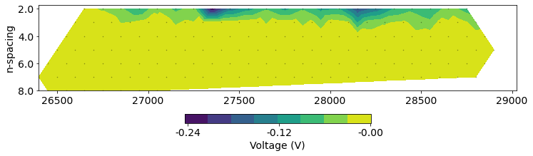
def plot_building_pseudosection(source_ind=0):
    """
    A plotting function to visualize how a pseudosection is built up.
    """

    fig, ax = plt.subplots(1, 1, figsize=(12, 4))
    mid_x, mid_z = dc.utils.source_receiver_midpoints(dc_data.survey)
    ax.plot(mid_x, mid_z, '.k', alpha=0.5)

    # plot the source location
    a_loc = dc_data_dict["a_locations"][source_ind]
    b_loc = dc_data_dict["b_locations"][source_ind]
    src_mid = (a_loc+b_loc)/2
    ax.plot(np.r_[a_loc, b_loc], np.r_[0, 0], 'C0.')
    ax.plot(src_mid, np.r_[0], 'C0x', ms=6)

    # plot the receiver locations
    m_locs = dc_data_dict["m_locations"][source_ind]
    n_locs = dc_data_dict["n_locations"][source_ind]
    rx_mid = (m_locs+n_locs)/2
    ax.plot(np.r_[m_locs, n_locs], np.zeros(2*len(m_locs)), 'C1.')
    ax.plot(rx_mid, np.zeros_like(m_locs), 'C1x', ms=6)

    # plot where the pseudosection points should be
    pseudo_x = (rx_mid + src_mid)/2.
    pseudo_z = -np.abs(rx_mid-src_mid)/2.

    ax.plot(np.r_[src_mid, pseudo_x], np.r_[0, pseudo_z], '-k', alpha=0.3)

    # draw lines to the points we are plotting
    for rx_x, px, pz in zip(rx_mid, pseudo_x, pseudo_z):
        ax.plot(np.r_[px, rx_x], np.r_[pz, 0], '-k', alpha=0.3)

    # these are the data corresponding to the source-receiver pairs we are looking at
    ax.plot(pseudo_x, pseudo_z, 'C2o')
    ax.set_xlabel("Northing (m)")
    ax.set_ylabel("n-spacing")

    ax.set_yticklabels([])
    ax.set_xlim([25900, 29300])
    ax.set_aspect(1.5)
ipywidgets.interact(
    plot_building_pseudosection,
    source_ind=ipywidgets.IntSlider(min=0, max=int(dc_data_dict["n_sources"])-1, value=0)
)Apparent resistivity
Our measured data are potential differences in units of volts. Both the geometry of the sources and receivers, as well as the geology, influence these values. Having both of these factors influence the values can make it challenging to make sense of the data. In order to translate them to something more interpretable, it is common to work with apparent resistivity values, which are derived by considering the potentials that would be measured if the earth were a half-space:
Where:
- is the apparent resistivity ( m)
- is the measured potential difference (V)
- is the source current (A)
- is the geometric factor which depends on the location of all four electrodes.
Pseudosections of the apparent resistivity are a valuable tool for QC'ing and processing the data. It is easier to spot outliers and see trends in the data than using plots of the potentials.
# plot psuedosection
fig, ax = plt.subplots(1, 1, figsize=(12, 4))
dc.utils.plot_pseudosection(
    dc_data, data_type="apparent resistivity",
    plot_type="contourf", data_location=True, ax=ax, cbar_opts={"pad":0.25}
)
ax.set_aspect(1.5)  # some vertical exxageration
ax.set_title(f"DC: {line} Pseudosection")
ax.set_xlabel("Northing (m)")
Text(0.5, 0, 'Northing (m)')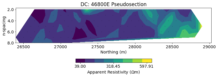
Histogram of our data
In addition to looking at a 2D pseudosection of the data, a histogram gives us an idea of the distribution of apparent resistivities. For more complex survey geometries (e.g. fully 3D), it is not always clear how to plot data in a pseudosection form, so histograms are a valueable tool for visualizing data and estimating a good background resistivity for the starting and reference models.
apparent_resistivity = dc.utils.apparent_resistivity(dc_data)fig, ax = plt.subplots(1, 1)
out = ax.hist(np.log10(apparent_resistivity), bins=30)
ax.set_xlabel("log$_{10}(\\rho_a)$")Text(0.5, 0, 'log$_{10}(\\rho_a)$')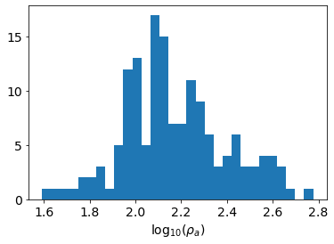
estimate a background model
# rho0 = 10**np.mean(np.log10(apparent_resistivity))
rho0 = np.median(apparent_resistivity)
rho0135.90619481429147Step 3: set up the forward simulation machinery
The DC resistivity equations
Now that we have a sense of our data, we will set up a forward simulation which is responsible for simulating predicted data given a model.
The equations we are solving are the steady-state Maxwell's equations:
Since the curl of the electric field is zero, we can represent it as a the gradient of a scalar potential .
Ohm's law relates the current density to the electric field through the resistivity, , in units of m (or equivalently through the electrical conductivity .
and assembling everything
Discretizing
In SimPEG, we use a Finite Volume approach to solving this partial differential equation (PDE). To do so, we define where each component of the equation lives on the mesh. Scalars can either be defined at cell centers or on nodes whereas vectors are defined on cell faces or edges. There are two discretizations implemented in SimPEG for the DC resistivity problem: Cell-Centered and Nodal. In both, we discretize physical properties (resistivity) at cell centers, and you can think of the resistivity filling that entire "lego-block". The difference between the two discretizations depends upon where we discretize the potential : either at the cell centers or the nodes. For this tutorial, we will use the Nodal discretization where
- : discretized at cell centers
- : discretized at nodes
- : discretized on cell edges

We will not go into the details here, but we highlight the importance of the boundary conditions. The Nodal discretization uses Neuman boundary conditions, which means that there is no flux of current through the boundary. Thus when we design our mesh, it needs to extend sufficiently far as to satisfy this condition.
For an overview of the derivation for the cell centered discretization, see the leading edge article Pixels and their Neighbors.
3.1 Design a Mesh
When designing a mesh, there are 3 main items to consider
minimum cell size:
- controls resolution
- typically ~4 per minimum electrode spacing
extent of the core domain:
- in the horizontal dimension: typically use the extent of the survey (or slightly beyond)
- in the vertical direction, we want the core region to extend to the depth to which we are sensitive to variations in physical properties. As a rule of thumb, this is typically a fraction of the maximum source-receiver separation
extent of the full modelling domain:
- need to satisfy boundary conditions!
- typically add ~the maximum source-receiver separation in each dimension
Here, we will use a TensorMesh, where each dimension can be defined with just a cell width.
A tensor in each dimension is enough to define the entire mesh.
For larger domains, we recommend using an TreeMesh. There are examples in the discretize documentation for creating QuadTree (2D) and OcTree (3D) meshes.
min_electrode_spacing = np.min(np.abs(survey.locations_a[:, 0] - survey.locations_b[:, 0]))
n_cells_per_spacing = 4

dx = min_electrode_spacing / n_cells_per_spacing
dz = min_electrode_spacing / n_cells_per_spacing

print(
    f"We will use a base mesh with {dx} m x {dz} m cells"
)
We will use a base mesh with 25.0 m x 25.0 m cells
core_domain_x = np.r_[
    survey.electrode_locations[:, 0].min(),
    survey.electrode_locations[:, 0].max()
]

core_domain_x
array([26000., 29200.])# find the maximum spacing between source, receiver midpoints
mid_ab = (survey.locations_a + survey.locations_b)/2
mid_mn = (survey.locations_m + survey.locations_n)/2
separation_ab_mn = np.abs(mid_ab - mid_mn)
max_separation = separation_ab_mn.max()
print(f"The maximum separation is {max_separation}m")
core_domain_z = np.r_[-max_separation/3., 0.]
core_domain_zThe maximum separation is 800.0m
array([-266.66666667, 0. ])n_core_extra = 4
n_core_x = np.ceil(np.diff(core_domain_x)/dx) + n_core_extra*2 # on each side
n_core_z = np.ceil(np.diff(core_domain_z)/dz) + n_core_extra # just below
padding_factor = 1.3
n_pad_x = 10
n_pad_z = 10hx = [(dx, n_pad_x, -padding_factor), (dx, n_core_x), (dx, n_pad_x, padding_factor)]
hz = [(dz, n_pad_z, -padding_factor), (dz, n_core_z)]
mesh = discretize.TensorMesh([hx, hz])
# origin of the mesh
mesh.x0 = np.r_[
-mesh.hx[:n_pad_x + n_core_extra].sum() + core_domain_x.min(),
-mesh.hy.sum()
]
meshfig, ax = plt.subplots(1, 1, figsize=(12, 4))
mesh.plotGrid(ax=ax)
ax.set_aspect(1.5)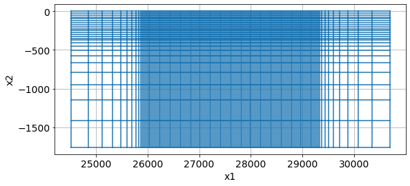
3.2: Construct the forward simulation
A simulation object contains everything we need to compute potentials given a resistivity model. It is instantiated with:
mesh: which discretizes the world and provides us with all of the differential operators
rhoMap: in SimPEG, the maps module provides flexibility for defining what our inversion model is. Each Map is a mathematical transform (that has a derivative - which we need in the inversion!). For example, the ExpMap takes the exponential of a model vector; we would define our model as log-resistivity. This is useful in electrical and electromagnetic inversions where we know that electrical resistivity should be strictly positive, and tends to vary logarithmically.

Similarly, mappings can be used to define active and inactive cells (for example if we have topography and don't want to invert for air-cells), or to define parametric models.
solver: A linear solver (e.g. LU) provided in the pymatsolver repository. Here we use Pardiso.
storeJ: for smaller problems, where we aren't memory limited, the inversion is faster if we store the sensitivity matrix rather than
# forward simulation
# Use Exponential Map: m = log(rho)
mapping = maps.ExpMap(mesh)

# Generate 2.5D DC problem
simulation_dc = dc.Simulation2DNodal(
    mesh, rhoMap=mapping, solver=Solver, survey=survey, storeJ=True
)
To check our mesh and forward simulation, we run a simulation over a half-space. The apparent resistivities we compute from the simulated data should be equal to the true half-space resistivity.
%%time

# run the forward simulation over the half-space & plot apparent resistivities
m0 = np.ones(mesh.nC) * np.log(rho0)
d0 = simulation_dc.make_synthetic_data(m0)
CPU times: user 1.03 s, sys: 72.7 ms, total: 1.11 s
Wall time: 373 ms
# plot psuedosection
fig, ax = plt.subplots(1, 1, figsize=(12, 4))

clim = np.r_[apparent_resistivity.min(), apparent_resistivity.max()]
dc.utils.plot_pseudosection(
    d0, data_type="apparent resistivity",  clim=clim,
    plot_type="contourf", data_location=True, ax=ax,
    cbar_opts={"pad":0.25}
)
ax.set_aspect(1.5)  # some vertical exxageration
ax.set_title(f"{line} Pseudosection")
ax.set_xlabel("Northing (m)")
Text(0.5, 0, 'Northing (m)')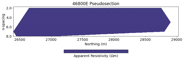
This next plot shows the percent error in the apparent resistivity. We want the error to be less than the errors in our data: 5% is common for assigning a percent uncertainty, so if the errors are below that, then we can be satisfied with our setup. If not, there are several things to check. In general (for nearly every geophysical survey):
- boundary conditions - does the mesh extend far enough?
- discretization near source and receivers - are we using fine-enough cells
- specifically for 2.5 DC: are we using enough filters (we will revisit this in the next notebook)
apparent_resistivity_m0 = dc.utils.apparent_resistivity(d0)
percent_error = (apparent_resistivity_m0 - rho0)/rho0*100

fig, ax = plt.subplots(1, 1)
ax.plot(separation_ab_mn[:, 0], percent_error, '.', alpha=0.4)
ax.set_xlabel("AB - MN separation")
ax.set_ylabel("percent difference (%)")
ax.set_title("Error in apparent resistivities")
ax.set_ylim(7*np.r_[-1, 1])
ax.grid(alpha=0.3)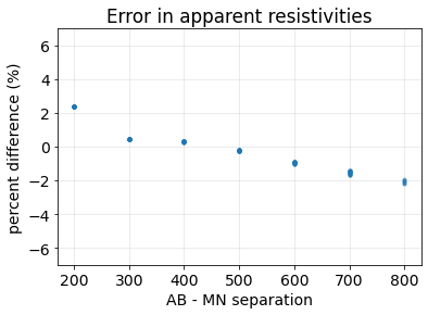
4. DC resistivity inversion
We forumlate the inverse problem as an optimization problem consisting of a data misfit and a regularization
where:
- is our inversion model - a vector containing the set of parameters that we invert for
- is the data misfit
- is the regularization
- is a trade-off parameter that weights the relative importance of the data misfit and regularization terms
- is our target misfit, which is typically set to where is the number of data (Parker, 1994) (or also see Oldenburg & Li (2005))
4.1 Data Misfit
The data misfit, , is often taken to be a weighted -norm, where the weights capture the noise model (eg. we want to assign higher weights and do a good job fitting data that we are confident are less noisy, and assign less weight / influence to data that are noisy). The norm is the correct norm to choose when noise is Gaussian (or approximately Gaussian, or if you have no additional information and assume it is Gaussian). An data misfit is captured mathematically by
where
- is a diagonal matrix with diagonal entries , where is an estimated standard deviation of the th datum.
- is the forward modelling operator that simulates predicted data given a model
- is the observed data
To instantiate the data misfit term, we provide a data object (which also has the associated uncertainties) along with a simulation which has the machinery to compute predicted data.
# set up the data misfit
dmisfit = data_misfit.L2DataMisfit(data=dc_data, simulation=simulation_dc)
4.2 Regularization
The inverse problem is an ill posed problem. There are multiple (actually infinitely many!) models that can fit the data. If we start by thinking about a linear problem , the matrix has more columns than rows, so it is not directly invertible (eg. see Matt Hall's Linear Inversion Tutorial). Here, we are dealing with a non-linear system of equations, but the principle is the same.
Thus, to choose from the infinitely many solutions and arrive at a sensible one, we employ a regularization: . Tikhonov regularization, which again uses -norms, is a standard choice (It has a few nice features: it is convex and easy to differentiate). It takes the form:
The first term is often referred to as the "smallness" as it measures the "size" of the model (in the sense). The matrix is generally taken to be a diagonal matrix that may contain information about the length scales of the model or be used to weight the relative importance of various parameters in the model. The scalar weights the relative importance of this term in the regularization.
Notice that we include a reference model (. Often this is defined as a constant value, but if more information is known about the background, that can be used to construct a reference model. Note that saying "I am not going to use a reference model" means that you are actually using , this is important to realize... in the inversion we demonstrate here, our model will be . If we set , then we are favoring models close to 1 m - which is quite conductive!
The second term is often referred to as the "smoothness". The matrix approximate the derivative of the model with respect to depth, and is hence a measure of how "smooth" the model is. The term weights its relative importance in the regularization.
The values have dimensions of ^2 as compared to . So if we choose our length scale to be 25m, the size of our finest cells and , then we set . In notebook 3-inversions-dc.ipynb. We will explore these choices further.
# Related to inversion
reg = regularization.Tikhonov(
    mesh,
    alpha_s=1./mesh.hx.min()**2,  # we will talk about these choices in notebook 3 on inversion
    alpha_x=1,
    alpha_y=1,  # since this is a 2D problem, the second dimension is "y"
)
Next, we assemble the data misfit and regularization into a statement of the inverse problem. We select an optimization method: in this case, a second-order Inexact Gauss Newton (see Nocedal and Wright, Ch 7). The inverse_problem then has all of the machinery necessary to evaluate the objective function and compute an update.
opt = optimization.InexactGaussNewton(maxIter=20, maxIterCG=20)
inv_prob = inverse_problem.BaseInvProblem(dmisfit, reg, opt)
4.3 Assemble the inversion
In SimPEG, we use directives to orchestrate updates during the inversion. The three we use below are
betaest: sets an initial value for by estimating the largest eigenvalue of and of and then taking their ratio. The value is then scaled by thebeta0_ratiovalue, so for example if you wanted the regularization to be ~10 times more important than the data misfit, then we would setbeta0_ratio=10beta_schedule: this reduces the value of beta during the course of the inversion. Particularly for non-linear problems, it can be advantageous to start off by seeking a smooth model which fits the regularization and gradually decreasing the influence of the regularization to increase the influence of the data.target: this directive checks at the end of each iteration if we have reached the target misfit. If we have, the inversion terminates, it not, it continues.
# directives
beta_est = directives.BetaEstimate_ByEig(beta0_ratio=1e0)
beta_schedule = directives.BetaSchedule(coolingFactor=4, coolingRate=2)
target = directives.TargetMisfit()

inv = inversion.BaseInversion(
    inv_prob, directiveList=[beta_est, beta_schedule, target]
)
4.4 Run the inversion!
# Run inversion
mopt = inv.run(m0)
SimPEG.InvProblem will set Regularization.mref to m0.
SimPEG.InvProblem is setting bfgsH0 to the inverse of the eval2Deriv.
***Done using same Solver and solverOpts as the problem***
model has any nan: 0
============================ Inexact Gauss Newton ============================
# beta phi_d phi_m f |proj(x-g)-x| LS Comment
-----------------------------------------------------------------------------
x0 has any nan: 0
0 2.82e+00 9.10e+03 0.00e+00 9.10e+03 3.11e+03 0
1 2.82e+00 1.39e+03 8.24e+01 1.62e+03 4.71e+02 0
2 7.06e-01 2.39e+02 1.95e+02 3.77e+02 1.08e+02 0 Skip BFGS
------------------------- STOP! -------------------------
1 : |fc-fOld| = 0.0000e+00 <= tolF*(1+|f0|) = 9.0964e+02
1 : |xc-x_last| = 5.1001e+00 <= tolX*(1+|x0|) = 3.0775e+01
0 : |proj(x-g)-x| = 1.0776e+02 <= tolG = 1.0000e-01
0 : |proj(x-g)-x| = 1.0776e+02 <= 1e3*eps = 1.0000e-02
0 : maxIter = 20 <= iter = 3
------------------------- DONE! -------------------------
# plot psuedosection
fig, ax = plt.subplots(2, 1, figsize=(12, 8))

clim = np.r_[apparent_resistivity.min(), apparent_resistivity.max()]

for a, data, title in zip(
    ax,
    [dc_data.dobs, inv_prob.dpred],
    ["true", "recovered"]
):
    dc.utils.plot_pseudosection(
        dc_data, dobs=data, data_type="apparent resistivity",
        plot_type="contourf", data_location=True, ax=a,
        cbar_opts={"pad":0.25}, clim=clim
    )
    a.set_title(title)


for a in ax:
    a.set_aspect(1.5)  # some vertical exxageration
    a.set_xlabel("Northing (m)")
    a.set_ylabel("Pseudo-depth")

plt.tight_layout()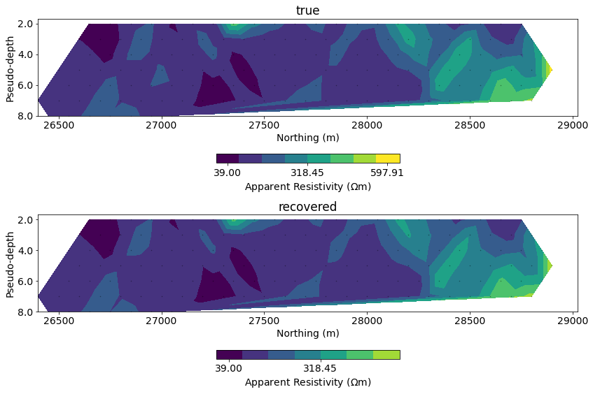
# plot misfit
fig, ax = plt.subplots(1, 1, figsize=(12, 4))

normalized_misfit = (inv_prob.dpred - dc_data.dobs) / dc_data.standard_deviation

dc.utils.plot_pseudosection(
    dc_data, dobs=normalized_misfit, data_type="misfit",
    plot_type="contourf", data_location=True, ax=ax,
    cbar_opts={"pad":0.25}
)

ax.set_title("DC misfit")
ax.set_aspect(1.5)  # some vertical exxageration
ax.set_xlabel("Northing (m)")
ax.set_ylabel("n-spacing")

cb_axes = plt.gcf().get_axes()[-1]
cb_axes.set_xlabel('normalized misfit')

plt.tight_layout()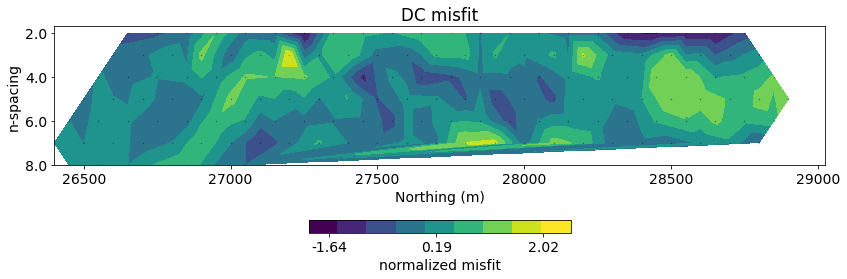
# run inversion, plot tikhonov curves

def load_leapfrog_geologic_section(filename="./century/geologic_section.csv"):
    """
    Load the geologic cross section.
    """
    fid = open(filename, 'r')
    lines = fid.readlines()
    data = []
    data_tmp = []
    for line in lines[2:]:
        line_data = (line.split(',')[:3])
        if 'End' in line:
            data.append(np.vstack(data_tmp)[:,[0, 2]])
            data_tmp = []
        else:
            data_tmp.append(np.array(line_data, dtype=float))
    return data
geologic_section = load_leapfrog_geologic_section()fig, ax = plt.subplots(1,1, figsize=(10, 5))
rho = (mapping*mopt)
out = mesh.plotImage(
rho, pcolorOpts={'norm':LogNorm(), 'cmap':'Spectral'}, ax=ax,
clim=(30, 1000)
)
for data in geologic_section:
ax.plot(data[:,0], data[:,1], 'k--', alpha=0.5)
ax.set_xlim(core_domain_x)
ax.set_ylim((-400, 0))
cb = plt.colorbar(out[0], fraction=0.05, orientation='horizontal', ax=ax, pad=0.2)
cb.set_label("Resistivity ($\Omega$m)")
ax.set_xlabel('Easting (m)')
ax.set_ylabel('Elevation (m)')
ax.set_aspect(1.5) # some vertical exxageration
plt.tight_layout()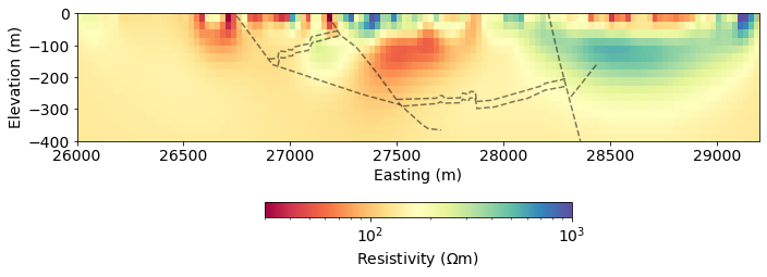
Compare to UBC results obtained 20 years ago(!)
mesh_ubc = discretize.TensorMesh.readUBC("century/46800E/468MESH.DAT")def read_ubc_model(filename, mesh_ubc=mesh_ubc):
"""
A function to read a UBC conductivity or chargeability model.
"""
values = np.genfromtxt(
filename, delimiter=' \n',
dtype=str, comments='!', skip_header=1
)
tmp = np.hstack([np.array(value.split(), dtype=float) for value in values])
model_ubc = discretize.utils.mkvc(tmp.reshape(mesh_ubc.vnC, order='F')[:,::-1])
return model_ubc
sigma_ubc = read_ubc_model("century/46800E/DCMODA.CON")
rho_ubc = 1./sigma_ubc
fig, ax = plt.subplots(2, 1, figsize=(10, 8))
rho = (mapping*mopt)
clim = (30, 1000)
out = mesh.plotImage(
rho, pcolorOpts={'norm':LogNorm(), 'cmap':'Spectral'}, ax=ax[0],
clim=clim
)
cb = plt.colorbar(out[0], fraction=0.05, orientation='horizontal', ax=ax[0], pad=0.2)
cb.set_label("Resistivity ($\Omega$m)")
ax[0].set_title("SimPEG")
out = mesh_ubc.plotImage(
rho_ubc, pcolorOpts={'norm':LogNorm(), 'cmap':'Spectral'}, ax=ax[1],
clim=clim
)
cb = plt.colorbar(out[0], fraction=0.05, orientation='horizontal', ax=ax[1], pad=0.2)
cb.set_label("Resistivity ($\Omega$m)")
ax[1].set_title("UBC")
for a in ax:
for data in geologic_section:
a.plot(data[:,0], data[:,1], 'k--', alpha=0.5)
a.set_xlim(core_domain_x)
a.set_ylim((-400, 0))
a.set_aspect(1.5) # some vertical exxageration
a.set_xlabel('Easting (m)')
a.set_ylabel('Elevation (m)')
plt.tight_layout()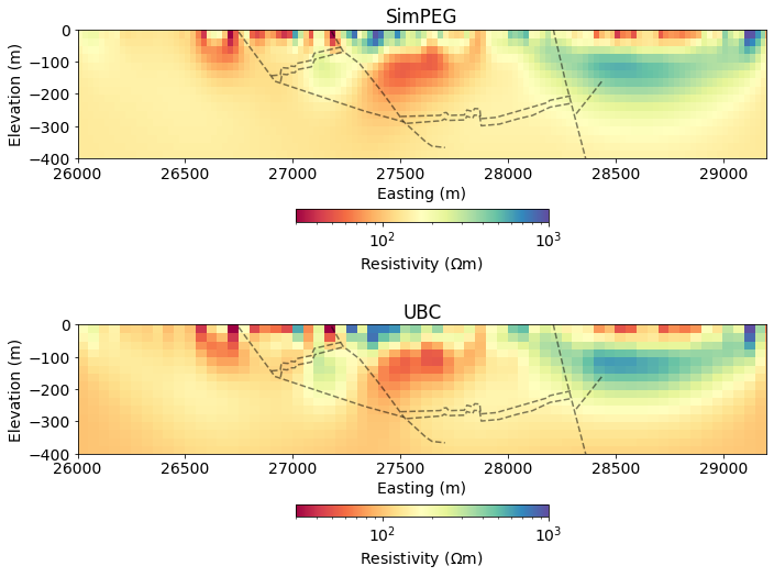
Induced Polarization
Induced Polarization (IP) surveys are sensitive to chargeability - the physical property which describes a material's tendency to become polarized and act like a capacitor.

The physical explanation for causes of chargeability are complex and are an active area of research. There are, however, two conceptual models that are insightful for characterizing the chareable behaviour of rocks: membrane polarization and electrode polarization.

Physically, the impact of chargeabile material causes the measured voltage to increase in the on-time, and after the current switch-off, the voltage decays. In the on-time, currents are primarily due to the potential difference made by a generator, and distorted by conductivity constrasts in the earth (DC-effects). In addition, polarization charges start to build, and reach steady state in the late on-time. After the current is switched off, all DC currents are immediately gone, but polarization charges remain and will start to discharge and generate a secondary voltage decay (IP).

For more background information on IP, including case histories, see the EM GeoSci pages on IP.
IP simulation
To simulate IP, we use a linearized model where we assume that the IP signals are due to a perturbation in electrical conductvity (inverse of resistivity)
with an IP datum written as
where the entries of J are the sensitivities for the DC resistivity problem
or in matrix form
For further discussion, see the derivation here
Step 5: Load the IP data
There are several ways to define IP data, for discussion, please see the reference page on IP data in em.geosci.xyz. For this survey, the data that we are provided are apparent chargeabilities (mV/V). This is analagous to apparent resistivity that we discussed for DC resistivity.
The file format and organization is identical to what we implemented for the DC data, so we can re-use that function to load our data into a dictionary.
ip_data_file = f"./century/{line}/{line[:-1]}IP.OBS"ip_data_dict = read_dcip_data(ip_data_file, verbose=False)The organization of an IP survey is very similar to the DC case. Here, we are calling sources and receivers from the ip module, and also specifying that the receivers are measring apparent chargeability data.
# initialize an empty list for each
source_list_ip = []

for i in range(ip_data_dict["n_sources"]):

    # receiver electrode locations in 2D
    m_locs = np.vstack([
        ip_data_dict["m_locations"][i],
        np.zeros_like(ip_data_dict["m_locations"][i])
    ]).T
    n_locs = np.vstack([
        ip_data_dict["n_locations"][i],
        np.zeros_like(ip_data_dict["n_locations"][i])
    ]).T

    # construct the receiver object
    receivers = ip.receivers.Dipole(
        locations_m=m_locs, locations_n=n_locs, data_type="apparent_chargeability"
    )

    # construct the source
    source = ip.sources.Dipole(
        location_a=np.r_[ip_data_dict["a_locations"][i], 0.],
        location_b=np.r_[ip_data_dict["b_locations"][i], 0.],
        receiver_list=[receivers]
    )

    # append the new source to the source list
    source_list_ip.append(source)
survey_ip = ip.Survey(source_list_ip)ip_data = Data(
survey=survey,
dobs=np.hstack(ip_data_dict["observed_data"]),
standard_deviation=np.hstack(ip_data_dict["standard_deviations"])
)# plot psuedosection
fig, ax = plt.subplots(1, 1, figsize=(12, 4))
ip.utils.plot_pseudosection(
ip_data, data_type="apparent chargeability",
plot_type="contourf", data_location=True, ax=ax,
)
ax.set_title(f"IP: {line} Pseudosection")
ax.set_aspect(1.5) # some vertical exxageration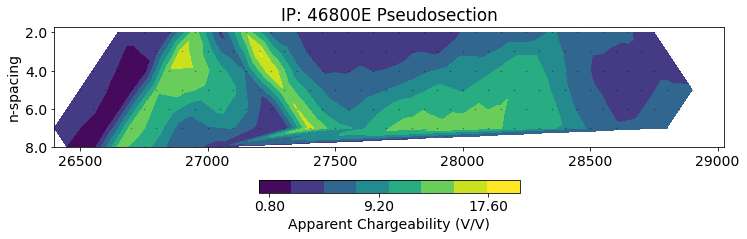
Step 6: Define the IP simulation
The general setup of an IP simulation is very similar to what we saw earlier for DC. Now, instead of inverting for resistivity (rho), we invert for chargeability (eta). The only additional parameter that is needed is the electrical resistivity (rho) from the DC inversion. This is used to construct the forward operator in the linear model of IP as described in the IP Simulation section above.
simulation_ip = ip.simulation_2d.Simulation2DNodal(
    mesh=mesh, solver=Solver, rho=np.exp(mopt),
    etaMap=maps.IdentityMap(mesh), survey=survey_ip,
    storeJ=True
)
Step 7: IP inversion
The setup for the IP inversion is very similar to what we did earlier for DC. The only change you will notice is that for the optimization, we are now using ProjectedGNCG: this is a Projected Gauss Newton with Conjugate Gradient (an iterative solver) optimization routine. It is similar to Inexact Gauss Newton but allows bound contstraints to be imposed. Here, we know that apparent chargeability is positive, so we use a lower bound of zero.
We do not use an ExpMap as we did for resistivity in the DC inversion because chargeability tends to vary on a linear scale.
dmisfit_ip = data_misfit.L2DataMisfit(data=ip_data, simulation=simulation_ip)

# Related to inversion
reg_ip = regularization.Tikhonov(
    mesh,
    alpha_s=1/mesh.hx.min()**2.,
    alpha_x=1.,
    alpha_y=1.,
)
opt_ip = optimization.ProjectedGNCG(
maxIter=20, maxIterCG=20, upper=np.inf, lower=0.
)inv_prob_ip = inverse_problem.BaseInvProblem(dmisfit_ip, reg_ip, opt_ip)Set a small starting model - this is often assumed to be zero (no chargeable material). Here, since we will be using bound constraints in the optimization, we use a small value to reduce challenges of "getting stuck" on the lower bound of zero.
m0_ip = 1e-3 * np.ones(mesh.nC)beta_est_ip = directives.BetaEstimate_ByEig(beta0_ratio=1e0)
beta_schedule_ip = directives.BetaSchedule(coolingFactor=2, coolingRate=1)
target_ip = directives.TargetMisfit()
inv_ip = inversion.BaseInversion(
inv_prob_ip, directiveList=[beta_est_ip, beta_schedule_ip, target_ip]
)# Run inversion
charge_opt = inv_ip.run(m0_ip)SimPEG.InvProblem will set Regularization.mref to m0.
SimPEG.InvProblem is setting bfgsH0 to the inverse of the eval2Deriv.
***Done using same Solver and solverOpts as the problem***
model has any nan: 0
=============================== Projected GNCG ===============================
# beta phi_d phi_m f |proj(x-g)-x| LS Comment
-----------------------------------------------------------------------------
x0 has any nan: 0
0 4.69e-02 4.45e+04 0.00e+00 4.45e+04 4.20e+02 0
1 2.34e-02 9.83e+02 5.26e+04 2.22e+03 3.78e+01 0
2 1.17e-02 3.92e+02 6.53e+04 1.16e+03 7.96e+00 0 Skip BFGS
3 5.86e-03 1.86e+02 7.70e+04 6.38e+02 7.64e+00 0 Skip BFGS
4 2.93e-03 1.03e+02 8.73e+04 3.59e+02 1.12e+01 0 Skip BFGS
------------------------- STOP! -------------------------
1 : |fc-fOld| = 0.0000e+00 <= tolF*(1+|f0|) = 4.4486e+03
0 : |xc-x_last| = 2.6671e+01 <= tolX*(1+|x0|) = 1.0624e-01
0 : |proj(x-g)-x| = 1.1396e+01 <= tolG = 1.0000e-01
0 : |proj(x-g)-x| = 1.1396e+01 <= 1e3*eps = 1.0000e-02
0 : maxIter = 20 <= iter = 5
------------------------- DONE! -------------------------
# plot misfit
fig, ax = plt.subplots(1, 1, figsize=(12, 4))

normalized_misfit = (inv_prob_ip.dpred - ip_data.dobs) / ip_data.standard_deviation

dc.utils.plot_pseudosection(
    ip_data, dobs=normalized_misfit, data_type="misfit",
    plot_type="contourf", data_location=True, ax=ax,
    cbar_opts={"pad":0.25}
)

ax.set_title("IP misfit")
ax.set_aspect(1.5)  # some vertical exxageration
ax.set_xlabel("Northing (m)")

cb_axes = plt.gcf().get_axes()[-1]
cb_axes.set_xlabel('normalized misfit')

plt.tight_layout()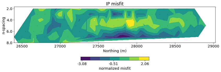
fig, ax = plt.subplots(1,1, figsize=(10, 5))
out = mesh.plotImage(
    charge_opt, pcolorOpts={'cmap':'Spectral_r'}, ax=ax,
    clim=(0, 30)
)
for data in geologic_section:
    ax.plot(data[:,0], data[:,1], 'k--', alpha=0.5)
ax.set_ylim((-400, 0))
ax.set_xlim(core_domain_x)
cb = plt.colorbar(out[0], label="chargeability", fraction=0.05, orientation='horizontal', ax=ax, pad=0.2)
ax.set_xlabel('Easting (m)')
ax.set_ylabel('Elevation (m)')
ax.set_aspect(1.5)
plt.tight_layout()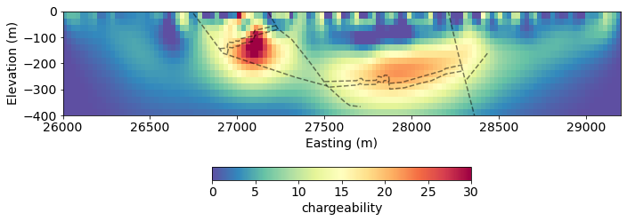
charge_ubc = read_ubc_model("century/46800E/IPMODA.CHG")fig, ax = plt.subplots(2, 1, figsize=(10, 8))
rho = (mapping*mopt)
clim = (0, 30)
out = mesh.plotImage(
charge_opt, pcolorOpts={'cmap':'Spectral_r'}, ax=ax[0],
clim=clim
)
cb = plt.colorbar(out[0], label="Chargeability", fraction=0.05, orientation='horizontal', ax=ax[0], pad=0.2)
ax[0].set_title("SimPEG")
out = mesh_ubc.plotImage(
charge_ubc, pcolorOpts={'cmap':'Spectral_r'}, ax=ax[1],
clim=clim
)
cb = plt.colorbar(out[0], label="Chargeability", fraction=0.05, orientation='horizontal', ax=ax[1], pad=0.2)
ax[1].set_title("UBC")
for a in ax:
for data in geologic_section:
a.plot(data[:,0], data[:,1], 'k--', alpha=0.5)
a.set_xlim(core_domain_x)
a.set_ylim((-400, 0))
a.set_aspect(1.5)
a.set_xlabel('Easting (m)')
a.set_ylabel('Elevation (m)')
plt.tight_layout()
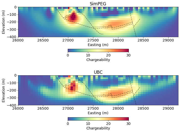
Homework ✏️
There are 6 lines of data in total for the century deposit. Can you invert them all?
Send us images of your results on Slack! We will share images of the UBC results in 1 week.
- Mutton, A. J. (2000). The application of geophysics during evaluation of the Century zinc deposit. GEOPHYSICS, 65(6), 1946–1960. 10.1190/1.1444878