Google Colab Setup¶

If you are using Google Colab to run this notebook, we assume you have already followed the Google Colab setup steps outlined here.

Because we are importing data, we need to "mount your Google Drive", which is where we tell this notebook to look for the data files. You will need to mount the Google Drive into each notebook.

Run the cell below if you are in Google Colab. If you are not in Google Colab, running the cell below will just return an error that says "No module named 'google'". If you get a Google Colab error that says "Unrecognised runtime 'geothrm'; defaulting to 'python3' Notebook settings", just ignore it.
Follow the link generated by running this code. That link will ask you to sign in to your google account (use the one where you have saved these tutorial materials in) and to allow this notebook access to your google drive.
Completing step 2 above will generate a code. Copy this code, paste below where it says "Enter your authorization code:", and press ENTER.

Congratulations, this notebook can now import data!

from google.colab import drive
drive.mount('/content/drive')

7. Injectivity index¶

The injectivity index is a measure of the amount of fluid the well can accept during injection. Specifically, it is the change in mass rate (t/hr) per change in pressure (bar), hence it has the units t/hr/bar.

If the well is destined to be used as an injection well, then the injectivity is a direct measure of the future well performance (though it must be corrected for different injectate temperatures).

If the well is destined to be used as a production well then the injectivity is used to give an indication of future productivity. Productivity index also has the units t/h/bar though it refers to the flow rate out of the well during production, divided by the pressure drop (pressure drawdown) downhole during production.

This notebook gives a workflow to:

Import and check data
Select the stable pressure values to use for each flow rate
Create the flow rate vs stable pressure plot (t/h vs bar)
Use linear regression to find the slope (t/h/bar)

8. Import, munge and check data¶

8.1 Use bespoke functions to import and munge data¶

Install all packages required for this notebook.

If you do not already have iapws in your environment, then you will need to pip install it. This will need to be done in Google Colab. If you followed the Anaconda setup instructions to make an environment with the environment.yml, then you will not need to do this.

!pip install iapws

Requirement already satisfied: iapws in /Users/stevejpurves/anaconda/anaconda3/envs/geothrm/lib/python3.7/site-packages (1.5.2)
Requirement already satisfied: scipy in /Users/stevejpurves/anaconda/anaconda3/envs/geothrm/lib/python3.7/site-packages (from iapws) (1.6.2)
Requirement already satisfied: numpy<1.23.0,>=1.16.5 in /Users/stevejpurves/anaconda/anaconda3/envs/geothrm/lib/python3.7/site-packages (from scipy->iapws) (1.20.2)

import iapws # steam tables
import openpyxl
import numpy as np
import pandas as pd
from scipy import stats
from datetime import datetime
import matplotlib.pyplot as plt
import matplotlib.dates as mdates
from IPython.display import Image
from ipywidgets import interactive, Layout, FloatSlider



def timedelta_seconds(dataframe_col, test_start):
    '''
    Make a float in seconds since the start of the test

    args:   dataframe_col: dataframe column containing datetime objects
            test_start: test start time formatted '2020-12-11 09:00:00'

    returns: float in seconds since the start of the test
    '''
    test_start_datetime = pd.to_datetime(test_start)
    list = []
    for datetime in dataframe_col:
        time_delta = datetime - test_start_datetime
        seconds = time_delta.total_seconds()
        list.append(seconds)
    return list



def read_flowrate(filename):
    ''' 
    Read PTS-2-injection-rate.xlsx in as a pandas dataframe and munge for analysis

    args: filename is r'PTS-2-injection-rate.xlsx'

    returns: pandas dataframe with local NZ datetime and flowrate in t/hr
    '''
    df = pd.read_excel(filename, header=1) 
    df.columns = ['raw_datetime','flow_Lpm']

    list = []
    for date in df['raw_datetime']:
        newdate = datetime.fromisoformat(date)
        list.append(newdate)
    df['ISO_datetime'] = list 

    list = []
    for date in df.ISO_datetime:
        newdate = pd.to_datetime(datetime.strftime(date,'%Y-%m-%d %H:%M:%S'))
        list.append(newdate)
    df['datetime'] = list

    df['flow_tph'] = df.flow_Lpm * 0.060

    df['timedelta_sec'] = timedelta_seconds(df.datetime, '2020-12-11 09:26:44.448')

    df.drop(columns = ['raw_datetime', 'flow_Lpm', 'ISO_datetime'], inplace = True)

    return df



def read_pts(filename):
    '''
    Read PTS-2.xlsx in as a Pandas dataframe and munge for analysis

    args: filename is r'PTS-2.xlsx'

    returns: Pandas dataframe with datetime (local) and key coloumns of PTS data with the correct dtype
    '''
    df = pd.read_excel(filename)

    dict = {
        'DEPTH':'depth_m',
        'SPEED': 'speed_mps',
        'Cable Weight': 'cweight_kg',
        'WHP': 'whp_barg',
        'Temperature': 'temp_degC',
        'Pressure': 'pressure_bara',
        'Frequency': 'frequency_hz'
    }
    df.rename(columns=dict, inplace=True)

    df.drop(0, inplace=True)
    df.reset_index(drop=True, inplace=True)

    list = []
    for date in df.Timestamp:
        newdate = openpyxl.utils.datetime.from_excel(date)
        list.append(newdate)
    df['datetime'] = list

    df.drop(columns = ['Date', 'Time', 'Timestamp','Reed 0',
       'Reed 1', 'Reed 2', 'Reed 3', 'Battery Voltage', 
       'PRT Ref Voltage','SGS Voltage', 'Internal Temp 1', 
       'Internal Temp 2', 'Internal Temp 3','Cal Temp', 
       'Error Code 1', 'Error Code 2', 'Error Code 3',
       'Records Saved', 'Bad Pages',], inplace = True)
    
    df[
        ['depth_m', 'speed_mps','cweight_kg','whp_barg','temp_degC','pressure_bara','frequency_hz']
    ] = df[
        ['depth_m','speed_mps','cweight_kg','whp_barg','temp_degC','pressure_bara','frequency_hz']
        ].apply(pd.to_numeric)
    
    df['timedelta_sec'] = timedelta_seconds(df.datetime, '2020-12-11 09:26:44.448')

    return df



def append_flowrate_to_pts(flowrate_df, pts_df):
    '''
    Add surface flowrate to pts data

    Note that the flowrate data is recorded at a courser time resolution than the pts data
    The function makes a linear interpolation to fill the data gaps
    Refer to bonus-combine-data.ipynb to review this method and adapt it for your own data

    Args:   flowrate and pts dataframes generated by the read_flowrate and read_pts functions

    Returns: pts dataframe with flowrate tph added
    
    '''
    flowrate_df = flowrate_df.set_index('timedelta_sec')
    pts_df = pts_df.set_index('timedelta_sec')
    combined_df = pts_df.join(flowrate_df, how = 'outer',  lsuffix = '_pts', rsuffix = '_fr')
    combined_df.drop(columns = ['datetime_fr'], inplace = True)
    combined_df.columns = ['depth_m', 'speed_mps', 'cweight_kg', 'whp_barg', 'temp_degC',
       'pressure_bara', 'frequency_hz', 'datetime', 'flow_tph']
    combined_df['interpolated_flow_tph'] = combined_df['flow_tph'].interpolate(method='linear')
    trimmed_df = combined_df[combined_df['depth_m'].notna()]
    trimmed_df.reset_index(inplace=True)
    return trimmed_df



def find_index(value, df, colname):
    '''
    Find the dataframe index for the exact matching value or nearest two values

    args:   value: (float or int) the search term
            df: (obj) the name of the dataframe that is searched
            colname: (str) the name of the coloum this is searched

    returns:  dataframe index(s) for the matching value or the two adjacent values
              rows can be called from a df using df.iloc[[index_number,index_number]]
    '''
    exactmatch = df[df[colname] == value]
    if not exactmatch.empty:
        return exactmatch.index
    else:
        lowerneighbour_index = df[df[colname] < value][colname].idxmax()
        upperneighbour_index = df[df[colname] > value][colname].idxmin()
        return [lowerneighbour_index, upperneighbour_index] 

    

def overview_fig(pts_df,flowrate_df,title=''):
    fig, (ax1, ax2, ax3, ax4, ax5, ax6) = plt.subplots(6, 1,figsize=(10,15),sharex=True)
    ax1.set_title(title,y=1.1,fontsize=15)

    ax1.plot(flowrate_df.datetime, flowrate_df.flow_tph, label='Surface pump flowrate', 
        c='k', linewidth=0.8, marker='.')
    ax1.set_ylabel('Surface flowrate [t/hr]')
    ax1.set_ylim(0,150)
    
    ax2.plot(pts_df.datetime, pts_df.depth_m, label='PTS tool depth', 
        c='k', linewidth=0.8)
    ax2.set_ylabel('PTS tool depth [m]')
    ax2.set_ylim(1000,0)
    
    ax3.plot(pts_df.datetime, pts_df.pressure_bara, label='PTS pressure', 
        c='tab:blue', linewidth=0.8)
    ax3.set_ylabel('PTS pressure [bara]')
    
    ax4.plot(pts_df.datetime, pts_df.temp_degC, label='PTS temperature', 
        c='tab:red', linewidth=0.8)
    ax4.set_ylabel('PTS temperature')
    
    ax5.plot(pts_df.datetime, pts_df.frequency_hz, label='PTS impeller frequency', 
        c='tab:green', linewidth=0.8)
    ax5.set_ylim(-30,30)
    ax5.set_ylabel('PTS impeller frequency [hz]')
    # 1 hz = 60 rpm

    ax6.plot(pts_df.datetime, pts_df.speed_mps, label='PTS tool speed', 
        c='tab:orange', linewidth=0.8)
    ax6.set_ylim(-2,2)
    ax6.set_ylabel('PTS tool speed [mps]')
    
    ax6.set_xlabel('Time [hh:mm]')
    plt.gca().xaxis.set_major_formatter(mdates.DateFormatter('%H:%M'))
    
    for ax in [ax1,ax2,ax3,ax4,ax5,ax6]:
        ax.grid()
    
    return plt

The cells below will take a little while to run because it includes all steps required to import and munge the data (i.e., everything we did in notebook 1).

# Use this method if you are running this notebook in Google Colab
# flowrate = read_flowrate(r'/content/drive/My Drive/T21-Tutorial-WellTestAnalysis-main/Data-FlowRate.xlsx')

# Use this method if you are running this notebook locally (Anaconda)
flowrate = read_flowrate(r'Data-FlowRate.xlsx')

# Use this method if you are running this notebook in Google Colab
# pts = read_pts(r'/content/drive/My Drive/T21-Tutorial-WellTestAnalysis-main/Data-PTS.xlsx')

# Use this method if you are running this notebook locally (Anaconda)
pts = read_pts(r'Data-PTS.xlsx')

We use surface pump flow rate and downhole pressure together for our analysis, so we append flow rate to our pts dataframe to make the method simpler. This is done using the append_flowrate_to_pts function from the collection of helper functions above.

pts = append_flowrate_to_pts(flowrate, pts)

8.2 Import stable temperature/pressure data for comparison¶

After drilling and injection testing, geothermal wells heat up over time. So for comparison, we have provided a temperature log acquired when the well had reached its stable condition.

# Use this method if you are running this notebook in Google Colab
# heating_37days = pd.read_csv(r'/content/drive/My Drive/T21-Tutorial-WellTestAnalysis-main/Data-Temp-Heating37days.csv') 

# Use this method if you are running this notebook locally (Anaconda)
heating_37days = pd.read_csv('Data-Temp-Heating37days.csv')

# Convert bar gauge to bar atmosphere

heating_37days['pressure_bara'] = heating_37days.pres_barg - 1

heating_37days.head(2)

8.3 Check the data¶

It is good practice to check your data after import.

You can use the Pandas methods listed in Section 2.1.1 (1-intro-and-data.ipynb) to check your data.

pts.head(2)

flowrate.head(2)

heating_37days.head(2)

We made the plot below to check that we have imported what we expected to import.

fig, (ax1, ax2) = plt.subplots(1, 2,figsize=(24,8),sharey=True)

ax1.scatter(pts.pressure_bara, pts.depth_m, c = pts.timedelta_sec, s = 5, linewidths = 0)

ax1.plot(heating_37days.pressure_bara, heating_37days.depth_m, c = 'k', label = 'Heating 37 days')

ax1.legend()

ax2.scatter(pts.datetime, pts.depth_m, c = pts.timedelta_sec, s = 5, linewidths = 0)

ax3 = ax2.twinx()
ax3.plot(flowrate.datetime, flowrate.flow_tph, 
    c='k', linestyle = '-', linewidth = 3, alpha = 0.3, 
    label='Surface pump flowrate')

ax1.set_ylim(1000,0)  # 940,400 
ax1.set_xlim(0,55)     # 20,500

ax1.set_xlabel('Pressure [bara]')
ax1.set_ylabel('Depth [m]')

ax2.set_xlabel('Time [hh:mm]')
ax2.xaxis.set_major_formatter(mdates.DateFormatter('%H:%M'))

ax3.set_ylabel('Flowrate [t/hr]')

for ax in [ax1, ax2]:
    ax.grid()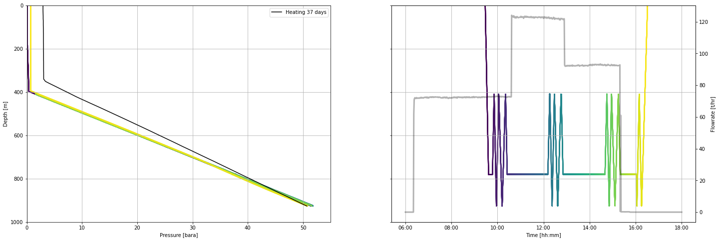

9. Pressure inside geothermal wells¶

Note that the pressure measured inside the well does not equate to the pressure in the reservoir. It varies depending on the liquid level and the density (temperature & phase) of the fluid inside the well. As the well heats up after drilling, pressure profiles will appear to pivot around a single point. That pressure of the pivot point equates to the reservoir pressure at the depth of pivoting.

10. Select the most stable pressure values for each flow rate¶

10.1 Interactive plot with ipywidgets¶

Use the interactive plot to select the times within the completion test program when the pressure down-hole is most likely to be stable for a given flow rate.

The most stable pressure is usually just after the pts tool returned to the programmed hanging depth that was for pressure transient after the well passes are complete and before the pump rate is changed.


min_timestamp = pts.timedelta_sec.iloc[0]
max_timestamp = pts.timedelta_sec.iloc[-1]

def subselect_plot(first_value, second_value, third_value):
    f,ax1 = plt.subplots(1,1, figsize = (20,6))
    ax1.plot(pts.timedelta_sec, pts.depth_m, c = 'k', label = 'PTS tool depth')
    ax2 = ax1.twinx()
    ax2.plot(flowrate.timedelta_sec, flowrate.flow_tph, c='k', linestyle = ':', label='Surface pump flowrate')
    ymin = pts.depth_m.min()
    ymax = pts.depth_m.max() + 100
    ax1.vlines(first_value, ymin, ymax, color='tab:green')
    ax1.vlines(second_value, ymin, ymax, color='tab:orange')
    ax1.vlines(third_value, ymin, ymax, color='tab:red')
    ax1.set_ylim(pts.depth_m.max() + 100, 0)
    ax1.set_xlabel('Time elapsed since the test started [sec]')
    ax2.set_ylabel('Surface pump flowrate [t/hr]')
    ax1.set_ylabel('PTS tool depth [mMD]')

result = interactive(subselect_plot,
         
         first_value = FloatSlider
         (
             value = (max_timestamp - min_timestamp)/6 + min_timestamp,
             description = '1st value',
             min = min_timestamp, 
             max = max_timestamp, 
             step = 10, 
             continuous_update=False,
             layout = Layout(width='80%'),
             ),
          
          second_value = FloatSlider
          (
             value = (max_timestamp - min_timestamp)/4 + min_timestamp, 
             description = '2nd value',
             min = min_timestamp, 
             max = max_timestamp, 
             step = 10, 
             continuous_update=False,
             layout = Layout(width='80%')
             ),

          third_value = FloatSlider
          (
             value = (max_timestamp - min_timestamp)/2 + min_timestamp, 
             description = '3rd value',
             min = min_timestamp, 
             max = max_timestamp, 
             step = 10, 
             continuous_update=False,
             layout = Layout(width='80%')
             )
)

display(result);

10.2 Call results from the interactive plot¶

After you place the 1st (green), 2nd (orange), and 3rd (red) line locations, run the cell below to call the results.

# extract pressure and flow rate at the marked points
print(
    'first_timestamp =',result.children[0].value, 
    '\nsecond_timestamp =', result.children[1].value, 
    '\nthird_timestamp =', result.children[2].value, 
    )

first_timestamp = 4257.648 
second_timestamp = 6386.472 
third_timestamp = 12772.944

10.3 Store analysis¶

Because result.children will change each time you move the sliders in the plot above or re-run this Jupyter Notebook, we copy-paste our selection below. This records your choice and will be the values you do the rest of the interpretation with.

Our selected data and some metadata¶

The third value was selected before the tool made passes because the pumps were shut off so quickly that it is difficult to reliably pick the value after the tool passes at this plot scale.

If we were concerned that the pressure was not stable before the logging passes, we could take the time to adjust the scale of our plot and pick the correct location.

# define a set of objects using our elapsed time
# we will use these to extract the data

first_timestamp = 3620.0 
second_timestamp = 12370.0 
third_timestamp = 18740.0

11. Generate an array of stable pressure and flow rate¶

Recall that we used the append_flowrate_to_pts function from our utilities.py in Section 8.1 above to append surface pump flow rate to our pts dataframe.

11.1 Make new dataframes containing the pts log values at our timestamps¶

Making our new dataframes is a two-step process:

Find the index value where the timestamp is either an exact match to the value we pass in or is the nearest neighbour above and below using the helper function at the start of this notebook
Make new dataframes using the .iloc method and the timestamp returned by step 1 (i.e., the find_index function)

first_pts = pts.iloc[find_index(first_timestamp, pts, 'timedelta_sec')]
second_pts = pts.iloc[find_index(second_timestamp, pts, 'timedelta_sec')]
third_pts = pts.iloc[find_index(third_timestamp, pts, 'timedelta_sec')]

first_pts

second_pts

third_pts

11.2 Make pressure and flow rate arrays¶

Now we either use the exact match value or the mean of the two neighbouring values to make an array of pressure and flow rate that we can use in our injectivity index analysis.

# make array of mean pressure values

list = []
for df in [first_pts, second_pts, third_pts]:
    mean_pressure = df['pressure_bara'].mean()
    list.append(mean_pressure)
pressure_array = np.array(list)

print('pressure data =', pressure_array)
print('object type =', type(pressure_array))

pressure data = [37.52142   37.7142575 37.6049115]
object type = <class 'numpy.ndarray'>

# make array of mean flowrate values

list = []
for df in [first_pts, second_pts, third_pts]:
    mean_flowrate = df['interpolated_flow_tph'].mean()
    list.append(mean_flowrate)
flowrate_array = np.array(list)

print('flowrate data =', flowrate_array)
print('object type =', type(flowrate_array))

flowrate data = [ 72.86231521 121.84291658  93.02511008]
object type = <class 'numpy.ndarray'>

12. Generate a linear regression to find injectivity index¶

The injectivity is a measure of total well capacity during injection. It is calculated from the change in pressure (bar) that occurs in response to changing the mass rate (t/hr) that is injected into the well.

If there is nothing unusual going on downhole, then we can find this with simple linear regression. There are many cases where a single linear model is not the best approach, such as where changes in pressure or thermal conditions in the well change the permeability. In these cases, a two-slope approach may be better.

12.1 Make the linear model¶

There are many ways to do a simple linear regression. We selected the stats.linregress method from Scipy because it is relatively simple to use. It's also fast because it is tooled specifically for our two-variable use case. The stats.linregress method returns the slope, intersect and R value that we need for our analysis.

linear_model = stats.linregress(pressure_array, flowrate_array) 

linear_model

LinregressResult(slope=254.48038077783218, intercept=-9475.995238015186, rvalue=0.9997019913953125, pvalue=0.015542479696471514, stderr=6.214136521958974, intercept_stderr=233.73612345134816)

# Define some sensibly named objects for reuse below

slope = linear_model[0]
intercept = linear_model[1]
rvalue = linear_model[2]

# Print a nicely formatted string describing of our model

print("The linear model for our data is y = {:.5} + {:.5} * pressure"
      .format(intercept, slope))

The linear model for our data is y = -9476.0 + 254.48 * pressure

12.2 Plot the results¶

f,ax = plt.subplots(1,1,figsize=(6,4))

ax.scatter(pressure_array, flowrate_array, 
           s=100, c='k', label = 'Data')

ax.plot(pressure_array, # x values
    slope * pressure_array + intercept, # use the model to generate y values
    color='tab:orange', linestyle='-', linewidth=4, alpha=0.5, label='Linear fit')


ax.set_title("Sample well injectivity index = {:} t/hr.bar".format(round(slope)))

#ax.set_ylim(0,130)
#ax.set_xlim(0,40)

ax.legend()
ax.set_ylabel('Rate [t/hr]')
ax.set_xlabel('Pressure [bara]')

Text(0.5, 0, 'Pressure [bara]')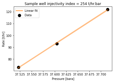

13. Interpreting injectivity index¶

13.1 Understanding the scale of injectivity index¶

Based on data from New Zealand geothermal fields, pre-eminent reservoir engineer Malcolm Grant determined that injectivity index forms a lognormal distribution with a median value around 20 t/hr.bar (Figure 5).

Image('https://raw.githubusercontent.com/ICWallis/T21-Tutorial-WellTestAnalysis/main/Figures/Figure5.png',width = 500,)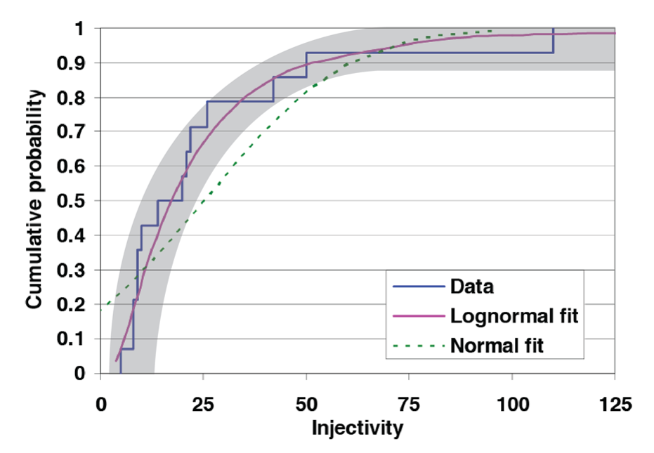

Figure 5: Like many natural phenomena, geothermal well injectivity has a lognormal distribution. Figure adapted from Grant (2008).

There is no 1:1 relationship between the injectivity index (II) and productivity index (PI) of a geothermal well. Each reservoir is subject to a unique set of conditions that influence the relationship between these indices, such as depth to the liquid level, and enthalpy.

The table below reflects a general rule of thumb to be used for a reservoir where the local relationship between II and PI has not already been established.

Permeability magnitude	II [t/hr.bar]
Very low permeability (near-conductive)	< 1
Poor permeability, usable in special cases	1 - 5
Likely productive	5 - 20
Median production well	20
Reliably economic production for well if T > 250 $^{\circ}$ C	20-50
High permeability	50 - 100
Very high permeability (unusual)	> 100

13.2 Injectivity index and temperature¶

The injectivity index is only truly valid for the injectate temperature at which it was measured (i.e., ambient temperature for completion testing). If you inject at a higher temperature (i.e., injection of separated geothermal water or condensate in operational injection wells), then the injectivity index will be less. Empirical corrections are available to adjust injectivity index for temperature - for more information refer to Siega et al. (2014)

14. Injectivity in our case study well¶

With an II of 252 t/hr.bar, our case study well is extremely permeable! Yah!

It is worth noting that as II increases, so does the level of uncertainty in the actual value. This is because the pressure changes resulting from the flow changes become so small. This is a good "problem" to have.

Cited references¶

Grant, M.A. (2008) Decision tree analysis of possible drilling outcomes to optimise drilling decisions: Proceedings, Thrity-Third Workshop of Geothermal Reservoir Engineering. Stanford University, CA.

Siega, C., Grant, M.A., Bixley, P. Mannington, W. (2014) Quantifying the effect of temperature on well injectivity: Proceedings 36th New Zealand Geothermal Workshop. Auckland, NZ.

Zarrouk, S.J. and McLean, K. (2019): Geothermal well test analysis: fundamentals, applications, and advanced techniques. 1st edition, Elsevier.

Licensed under the Apache License, Version 2.0

T21 - Geothermal Well Test Analysis

Temperature log data extraction and interpretation