Transform 2021: GemPy Workshop¶

Table of Content¶

Installation - Welcome
Basics Refresher (~25 mins)
Intro to subsurface (~ 25 mins)
Break (~ 10 mins)
subsurface to gempy (~ 25 mins)
Dealing with complexity (~ 25 mins)

Installation¶

https://docs.conda.io/en/latest/miniconda.html
Open conda prompt (Windows) or terminal (Linux/MacOS)
$ conda create --name gempy-tutorial python==3.8.5
Activate enviromet: $ conda activate gempy-tutorial
Installing gempy: https://docs.gempy.org/installation.html
clone the repo: git clone https://github.com/cgre-aachen/gempy_workshops.git
$ conda install jupyter notebook
$ jupyter notebook

Part I: Your first model (refresher)¶

# List of relative paths used during the workshop
path_to_well_png     = '../../common/basics/data/wells.png'
path_to_checkpoint_1 = '../../common/basics/checkpoints/checkpoint1.pickle'
path_to_checkpoint_2 = '../../common/basics/checkpoints/checkpoint2.pickle'
upgrade_pickles = False

# Importing GemPy
import gempy as gp

# Importing aux libraries
from ipywidgets import interact
import numpy as np
import matplotlib.image as mpimg

# Embedding matplotlib figures in the notebooks
%matplotlib qt5

Initializing the model... But first a word about Grids:¶

The first step to create a GemPy model is create a gempy.Model object that will contain all the other data structures and necessary functionality. In addition for this example we will define a regular grid since the beginning. This is the grid where we will interpolate the 3D geological model.

GemPy is based on a meshless interpolator. In practice this means that we can interpolate any point in a 3D space. However, for convenience, we have built some standard grids for different purposes. At the current day the standard grids are:

Regular grid: default grid mainly for general visualization
Custom grid: GemPy's wrapper to interpolate on a user grid
Topography: Topographic data use to be of high density. Treating it as an independent grid allow for high resolution geological maps
Sections: If we predefine the section 2D grid we can directly interpolate at those locations for perfect, high resolution estimations
Center grids: Half sphere grids around a given point at surface. This are specially tuned for geophysical forward computations

For now we will use a 2.5D regular grid

geo_model = gp.create_model('Transform-2021')
geo_model = gp.init_data(geo_model,
                         extent= [0, 791, 0, 200, -582, 0], # of the regular grid
                         resolution=[100, 10, 100])         # of the regular grid

Active grids: ['regular']

GemPy core code is written in Python. However for efficiency and gradient based machine learning most of heavy computations happen in optimize compile code, either C or CUDA for GPU.

To do so, GemPy rely on the library Theano. To guarantee maximum optimization Theano requires to compile the code for every Python kernel. The compilation is done by calling the following line at any point (before computing the model):

gp.set_interpolator(
    geo_model,
    output=['geology'], # In built outputs. More about this later on
    theano_optimizer='fast_compile') # alternatives: 'fast_run' or
                                     # check http://deeplearning.net/software/theano/tutorial/modes.html

Setting kriging parameters to their default values.
Compiling theano function...
Level of Optimization:  fast_compile
Device:  cpu
Precision:  float64
Number of faults:  0
Compilation Done!
Kriging values: 
                        values
range              1002.20008
$C_o$            23914.404762
drift equations           [3]

<gempy.core.interpolator.InterpolatorModel at 0x28f750a6fa0>

Creating figure:¶

GemPy uses matplotlib and pyvista for 2d and 3d visualization of the model respectively. One of the design decisions of GemPy is to allow real time construction of the model. What this means is that you can start adding input data and see in real time how the 3D surfaces evolve. Lets initialize the visualization windows.

The first one is the 2d figure. Just place the window where you can see it (maybe move the jupyter notebook to half screen and use the other half for the renderers).

p2d = gp.plot_2d(geo_model, section_names=None,
                 direction=None, cell_number=None)
p2d.fig

<Figure size 640x480 with 0 Axes>

Add model section¶

In the 2d renderer we can add several cross section of the model. In this case, for simplicity sake we are just adding one perpendicular to y.

import matplotlib.pyplot as plt
# In this case perpendicular to the y axes
ax = p2d.add_section(cell_number=1, direction='y')
p2d.fig

Loading cross-section image:¶

Remember that gempy is simply using matplotlib and therefore the ax object created above is a standard matplotlib axes.

Lets load an image with the information of couple of boreholes

# Reading image
img = mpimg.imread(path_to_well_png)
# Plotting it inplace
ax.imshow(img, origin='upper', alpha=.8, extent = (0, 791, -582,0))
p2d.fig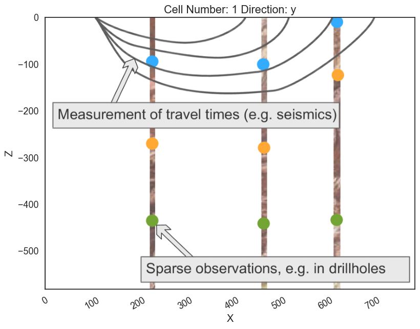

We can do the same in 3D through pyvista and vtk rendering.

Click the qt5 button Back (+Y) to have the same view as in the 2D viewer:

p3d = gp.plot_3d(geo_model, plotter_type='background', notebook=False)

# Small function to display screenshots in the notebook
def plot_pyvista_to_notebook(pyvista_plot):
    img = pyvista_plot.screenshot()
    fig = plt.Figure(frameon=False)
    ax_suplot= fig.add_subplot()
    ax_suplot.axis("off")
    ax_suplot.imshow(img)
    return fig

plot_pyvista_to_notebook(p3d.p)

Building the model¶

Now that we have the model initialize and the 2D and 3D render in place we can start the construction of the geological model.

Surfaces¶

GemPy is a surface based interpolator. This means that all the input data we add has to be refereed to a surface. The surfaces always mark the bottom of a unit.

By default GemPy surfaces are empty:

geo_model.surfaces

If we do not care about the names and we just want to interpolate a surface we can use. It is important to notice that the bottom most layer will be considered always basement and therefore not interpolated. Still we can add values or change the color of that "surface" (for lack of a better name) to populate the lower most volume.

# Default surfaces:
geo_model.set_default_surfaces()

We will see more about data structures below.

Now we can start adding data. GemPy input data consist on surface points and orientations (perpendicular to the layers). The 2D plot gives you the X and Z coordinates when hovering the mouse over. We can add a surface point as follows:

# Add a point. If idx is None, next available index will be used. Here we pass it
# explicitly for consistency
geo_model.add_surface_points(X=223, Y=0.01, Z=-94,
                             surface='surface1', idx=0)

# Plot in 2D
p2d.plot_data(ax, cell_number=11)

# Plot in 3D
p3d.plot_data()

p2d.fig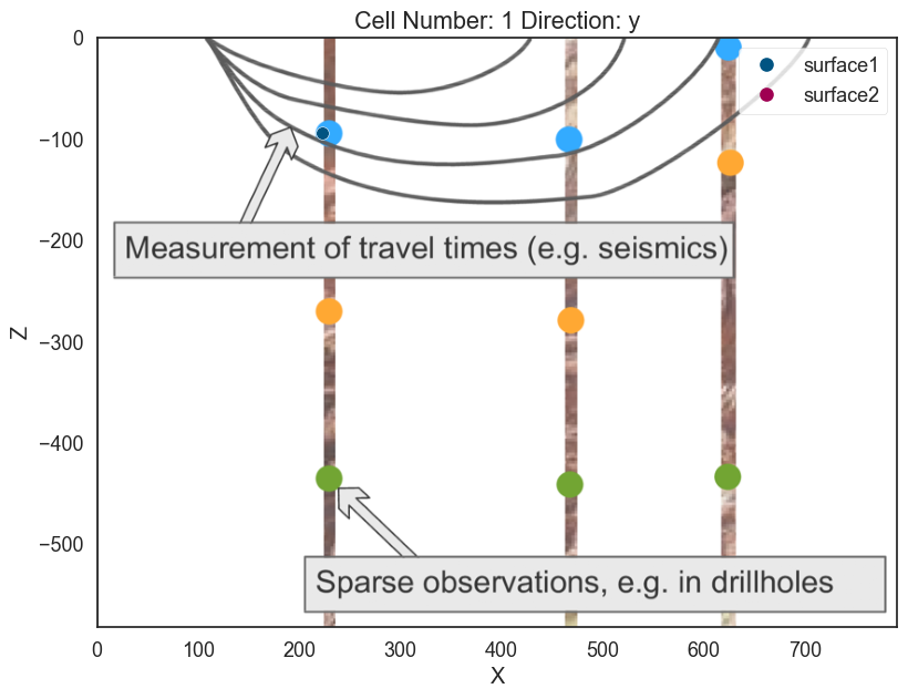

plot_pyvista_to_notebook(p3d.p)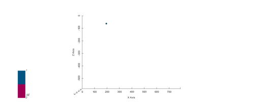

Now we can add the other two points of the layer:

# Add points
geo_model.add_surface_points(X=458, Y=0, Z=-107, surface='surface1', idx=1)
geo_model.add_surface_points(X=612, Y=0, Z=-14, surface='surface1', idx=2)

# Plotting
p2d.plot_data(ax, cell_number=11)
p3d.plot_surface_points()

(vtkmodules.vtkRenderingOpenGL2.vtkOpenGLActor)0000028F0117BE20

p2d.fig

plot_pyvista_to_notebook(p3d.p)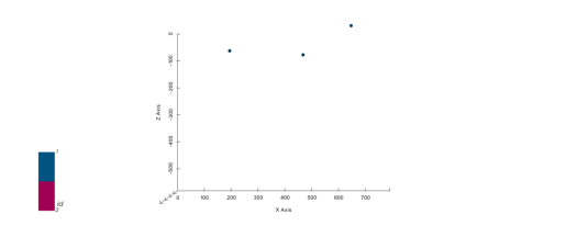

geo_model.surface_points

The minimum amount of input data to interpolate anything in gempy is:

a) 2 surface points per surface

b) One orientation per series.

Lets add an orientation anywhere in space:

# Adding orientation
geo_model.add_orientations(X=350, Y=0, Z=-300, surface='surface1',
                           pole_vector= (0,0,1))
p2d.plot_data(ax, cell_number=5)
p3d.plot_data()

p2d.fig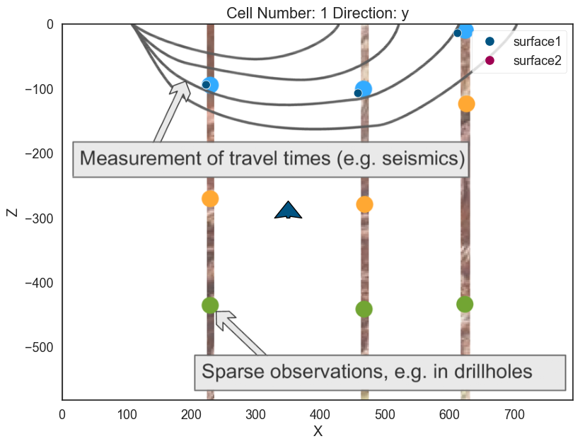

plot_pyvista_to_notebook(p3d.p)

Now we have enough data to finally interpolate!

gp.compute_model(geo_model)


Lithology ids 
  [2. 2. 2. ... 2. 2. 2.]

That is, we have interpolated the 3D surface. We can visualize with:

# In 2D
p2d.plot_contacts(ax, cell_number=5)

# In 3D
p3d.plot_surfaces()
p3d.plot_structured_grid()

[StructuredGrid (0x28f067aba00)
   N Cells:	88209
   N Points:	100000
   X Bounds:	3.955e+00, 7.870e+02
   Y Bounds:	1.000e+01, 1.900e+02
   Z Bounds:	-5.791e+02, -2.910e+00
   Dimensions:	100, 10, 100
   N Arrays:	2,
 <matplotlib.colors.ListedColormap at 0x28f067a20a0>]

p2d.fig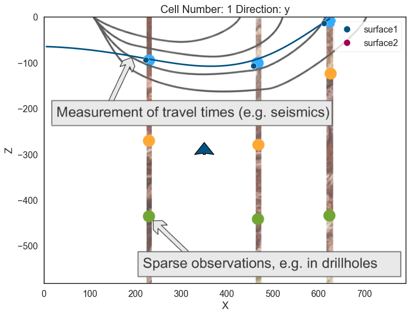

plot_pyvista_to_notebook(p3d.p)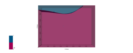

geo_model.solutions.lith_block

array([2., 2., 2., ..., 2., 2., 2.])

geo_model.surfaces

Congratulations! You have learnt how to create a surface. From here on, we will learn how to combine multiple surfaces to little by little construct a full realize 3D structural model.

Intermission: GemPy data classes¶

GemPy depends on multiple data objects to store all the data structures necessary to construct an structural model. To keep all the necessary objects in sync the class gempy.ImplicitCoKriging (which geo_model is instance of) will provide the necessary methods to update these data structures coherently.

At current state (gempy 2.2), the data classes are:

gempy.SurfacePoints
gempy.Orientations
gempy.Surfaces
gempy.Stack (combination of gempy.Series and gempy.Faults)
gempy.Grid
gempy.AdditionalData
gempy.Solutions

Today we will look into details only some of these classes but what is important to notice is that you can access these objects as follows:

# The default surfaces once again
geo_model.surfaces

# Also the surface points
geo_model.surface_points

# Orientations
geo_model.orientations

# To find the location of the surface we just plot
geo_model.solutions.vertices

[array([[  3.955     ,  10.        , -64.28490875],
        [  3.955     ,  30.        , -64.3000058 ],
        [ 11.865     ,  10.        , -64.6319632 ],
        ...,
        [624.85240288, 110.        ,  -2.91      ],
        [623.23234711, 130.        ,  -2.91      ],
        [621.12407188, 150.        ,  -2.91      ]])]

# The grid values:
geo_model.grid, len(geo_model.grid.values)

(Grid Object. Values: 
 array([[   3.955,   10.   , -579.09 ],
        [   3.955,   10.   , -573.27 ],
        [   3.955,   10.   , -567.45 ],
        ...,
        [ 787.045,  190.   ,  -14.55 ],
        [ 787.045,  190.   ,   -8.73 ],
        [ 787.045,  190.   ,   -2.91 ]]),
 100000)

# And its correspondent ids:
geo_model.solutions.lith_block, len(geo_model.solutions.lith_block)

(array([2., 2., 2., ..., 2., 2., 2.]), 100000)

Adding more layers¶

Exercise: So far we only need 2 units defined. The cross-section image that we load have 4 however. Lets add two layers more:

Layer 2¶

First we need to add some more layers.

# We can add already two extra surfaces
geo_model.add_surfaces(['surface3', 'basement'])

# Your code here:
geo_model.add_surface_points(X=225, Y=0, Z=-269, surface='surface2', idx=3)
geo_model.add_surface_points(X=459, Y=0, Z=-279, surface='surface2', idx=4)

#--------------------
# Plot data
p2d.plot_data(ax)
p3d.plot_data()

# Compute model
gp.compute_model(geo_model)

# Plot 2D
p2d.plot_lith(ax, cell_number=5)
p2d.plot_contacts(ax, cell_number=5)

# Plot 3D
p3d.plot_surfaces()
p3d.plot_structured_grid(opacity=.2, annotations = {1: 'surface1', 2:'surface2', 3:'surface3'})

[StructuredGrid (0x28f067aba00)
   N Cells:	88209
   N Points:	100000
   X Bounds:	3.955e+00, 7.870e+02
   Y Bounds:	1.000e+01, 1.900e+02
   Z Bounds:	-5.791e+02, -2.910e+00
   Dimensions:	100, 10, 100
   N Arrays:	2,
 <matplotlib.colors.ListedColormap at 0x28f011764f0>]

p2d.fig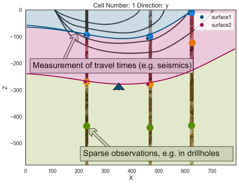

plot_pyvista_to_notebook(p3d.p)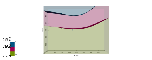

Layer 3¶

# Your code here:
# Add points
geo_model.add_surface_points(X=225, Y=0, Z=-439, surface='surface3')
geo_model.add_surface_points(X=464, Y=0, Z=-456, surface='surface3')
geo_model.add_surface_points(X=619, Y=0, Z=-433, surface='surface3')

# Compute model
gp.compute_model(geo_model)

# Plotting
p2d.plot_data(ax, cell_number=5)
p2d.plot_lith(ax, cell_number=5)
p2d.plot_contacts(ax, cell_number=5)

p3d.plot_surfaces()
p3d.plot_structured_grid(opacity=.2, annotations = {1: 'surface1', 2:'surface2', 3:'surface3', 4:'basement'})
p3d.plot_data()
# ------------------

p2d.fig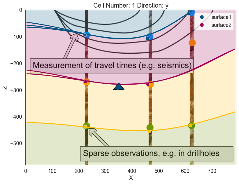

plot_pyvista_to_notebook(p3d.p)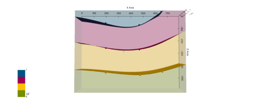

# Showing scalar field
scalar = gp.plot_2d(geo_model, show_scalar=True, series_n=0)
scalar.fig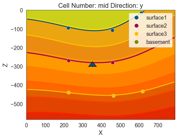

Intermission: GemPy data structures: Surfaces Points, Orientations and surfaces¶

On GemPy each surface is not independent of each other. Some surfaces will be subparallel to each other while other surfaces will define a fault plane where an offset may occur.

In order to account for all possible combinations, we use categories (in many instances literal pandas.CategoricalDtype) and ordered pandas.Dataframes. Let's take a look at gempy.SurfacePoints:

geo_model.surface_points

As we can see each point belong to a given surface. If now we look at the gempy.Surface object:

geo_model.surfaces

Here we can find the properties related to a each surface. Special attention to the column series. At the moment all surfaces belong to the same series and therefore they will be interpolated together in that characteristic subparallel pattern.

Now we will see how by playing with the series we can define unconformities and faults

Checkpoint: Next cell will load the model from disk to the necessary state to continue.

geo_model = gp.load_model_pickle(path_to_checkpoint_1)

# Default plotting setting
p2d = gp.plot_2d(geo_model)
ax = p2d.axes[0]
# Reading image
img = mpimg.imread('wells.png')
# Plotting it inplace
ax.imshow(img, origin='upper', alpha=.8, extent = (0, 791, -582,0))
p3d = gp.plot_3d(geo_model, plotter_type='background')

Unconformities and Faults:¶

So far the model is simply a depositional unit. GemPy allows for unconformities and faults to build complex models. This input is given by categorical data. In general:

Geometric Data (surface points/ orientations) <belong to< surface <belong to< series

And series can be a fault---i.e. offset the rest of surface--- or not. We are going to show how to add a fault as an example.

First we need to add a series:

Erosion¶

geo_model.add_features('Discontinuity')

Now there are two different series/features but not a surface that belong to it. Therefore, we also need to add a new surface:

geo_model.add_surfaces('discontinuity1')

Linking series/feature with surface:

gp.map_stack_to_surfaces(geo_model, {'Discontinuity':'discontinuity1'})

Notice that by default it is defining an erosion.

geo_model.reorder_features(['Discontinuity', 'Default series'])

geo_model.surfaces

Now we can just add input data as before (remember the minimum amount of input data to compute a model):

# Add input data of the fault
geo_model.add_surface_points(X=550, Y=0, Z=-30, surface='discontinuity1')
geo_model.add_surface_points(X=650, Y=0, Z=-200, surface='discontinuity1')
geo_model.add_orientations(X=600, Y=0, Z= -100, surface='discontinuity1',
                           pole_vector=(.3,0,.3))
# Plot
p2d.remove(ax)
p2d.plot_data(ax, cell_number=5)
p3d.remove_actor(p3d.regular_grid_actor) # Removing the previous regular grid because
                                         # we are changing the colors and gets messy
p3d.plot_data()

If we compute now the model the purple plane will erode the previous surfaces and layers:

# Compute
gp.compute_model(geo_model)

# Plot
p2d.remove(ax)
p2d.plot_data(ax, cell_number=5)
p2d.plot_lith(ax, cell_number=5)
p2d.plot_contacts(ax, cell_number=5)

p3d.plot_data()
p3d.plot_surfaces()
p3d.plot_structured_grid(opacity=.2, annotations = {2: 'surface1', 3:'surface2',
                                                    4:'surface3', 5:'basement'})

[StructuredGrid (0x28f067aba00)
   N Cells:	88209
   N Points:	100000
   X Bounds:	3.955e+00, 7.870e+02
   Y Bounds:	1.000e+01, 1.900e+02
   Z Bounds:	-5.791e+02, -2.910e+00
   Dimensions:	100, 10, 100
   N Arrays:	3,
 <matplotlib.colors.ListedColormap at 0x28f064fa490>]

p2d.fig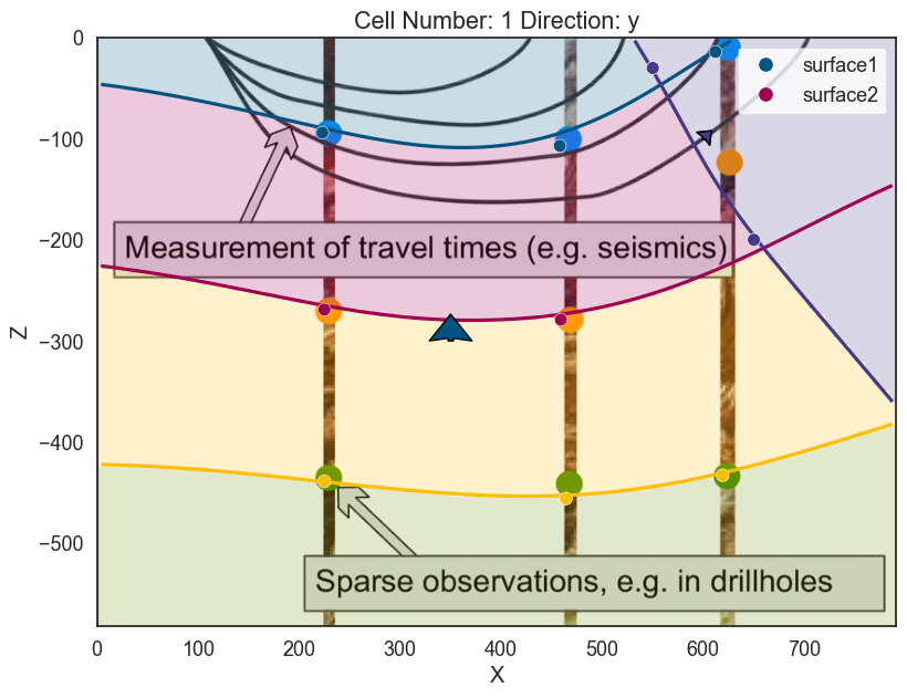

plot_pyvista_to_notebook(p3d.p)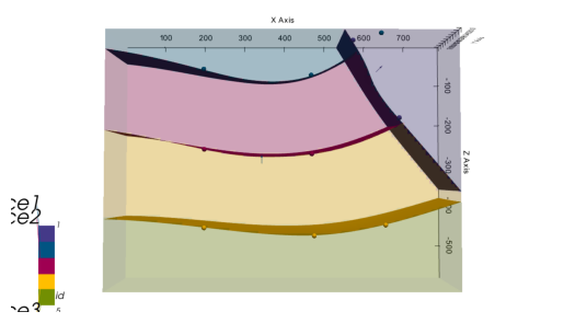

geo_model.stack

Onlap¶

If the relation should be onlap we just need to change the type of series/feature of discontinuity

geo_model.set_bottom_relation('Discontinuity', 'Onlap')


# %%
# Compute
gp.compute_model(geo_model)

# Plot
p2d.remove(ax)
p2d.plot_data(ax, cell_number=5)
p2d.plot_lith(ax, cell_number=5)
p2d.plot_contacts(ax, cell_number=5)

p3d.plot_data()
p3d.plot_structured_grid(opacity=.2, annotations = {2: 'surface1', 3:'surface2',
                                                    4:'surface3', 5:'basement'})

w:\miniconda\envs\gempy-tutorial\lib\site-packages\gempy\core\solution.py:353: UserWarning: Surfaces not computed due to: No surface found at the given iso value.. The surface is: Series: No surface found at the given iso value.; Surface Number:2
  warnings.warn('Surfaces not computed due to: ' + str(
w:\miniconda\envs\gempy-tutorial\lib\site-packages\gempy\core\solution.py:353: UserWarning: Surfaces not computed due to: No surface found at the given iso value.. The surface is: Series: No surface found at the given iso value.; Surface Number:3
  warnings.warn('Surfaces not computed due to: ' + str(

[StructuredGrid (0x28f067aba00)
   N Cells:	88209
   N Points:	100000
   X Bounds:	3.955e+00, 7.870e+02
   Y Bounds:	1.000e+01, 1.900e+02
   Z Bounds:	-5.791e+02, -2.910e+00
   Dimensions:	100, 10, 100
   N Arrays:	3,
 <matplotlib.colors.ListedColormap at 0x28f06855ca0>]

p2d.fig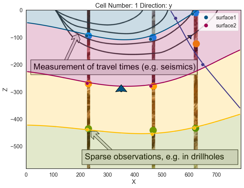

plot_pyvista_to_notebook(p3d.p)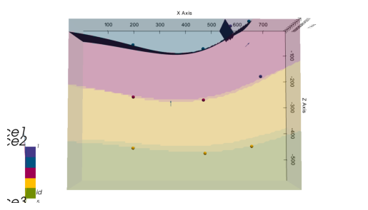

Fault¶

Then define that is a fault. It is possible to do this either by the set_bottom_relation method or set_is_fault.

geo_model.set_is_fault('Discontinuity')

And now is computing as before:

# Compute
gp.compute_model(geo_model)

# Plot
p2d.remove(ax)
p2d.plot_data(ax, cell_number=5)
p2d.plot_lith(ax, cell_number=5)
p2d.plot_contacts(ax, cell_number=5)

p3d.plot_data()
p3d.plot_surfaces()
p3d.plot_structured_grid(opacity=.2, annotations = {2: 'surface1', 3:'surface2',
                                                    4:'surface3', 5:'basement'})

[StructuredGrid (0x28f067aba00)
   N Cells:	88209
   N Points:	100000
   X Bounds:	3.955e+00, 7.870e+02
   Y Bounds:	1.000e+01, 1.900e+02
   Z Bounds:	-5.791e+02, -2.910e+00
   Dimensions:	100, 10, 100
   N Arrays:	3,
 <matplotlib.colors.ListedColormap at 0x28f0683dee0>]

By using multiple series/features instead of having folding layers we can have sharp interfaces. This opens

Additional features:¶

Over the years we have built a bunch of assets integrate with gempy. Here we will show some of them:

Topography¶

GemPy has a built-in capabilities to read and manipulate topographic data (through gdal). To show an example we can just create a random topography:

## Adding random topography
geo_model.set_topography(source='random',
                         fd=1.9, d_z=np.array([-150, 0]),
                         resolution=np.array([200,200]))

Active grids: ['regular' 'topography']

Grid Object. Values: 
array([[   3.955     ,   10.        , -579.09      ],
       [   3.955     ,   10.        , -573.27      ],
       [   3.955     ,   10.        , -567.45      ],
       ...,
       [ 791.        ,  197.98994975,  -54.02924024],
       [ 791.        ,  198.99497487,  -54.473154  ],
       [ 791.        ,  200.        ,  -54.83210375]])

The topography can we visualize in both renderers:

p2d.plot_topography(ax, cell_number=5)
p3d.plot_topography(scalars='topography')

(vtkmodules.vtkRenderingOpenGL2.vtkOpenGLActor)0000028F0037F280

But also allows us to compute the geological map of an area:

gp.compute_model(geo_model)
p3d.plot_surfaces()
p3d.plot_topography()

w:\miniconda\envs\gempy-tutorial\lib\site-packages\gempy\core\solution.py:174: VisibleDeprecationWarning: Creating an ndarray from ragged nested sequences (which is a list-or-tuple of lists-or-tuples-or ndarrays with different lengths or shapes) is deprecated. If you meant to do this, you must specify 'dtype=object' when creating the ndarray
  self.geological_map = np.array(

(vtkmodules.vtkRenderingOpenGL2.vtkOpenGLActor)0000028F064B6220

p3d.plot_structured_grid()

[UnstructuredGrid (0x28f0037f580)
   N Cells:	80576
   N Points:	92702
   X Bounds:	3.955e+00, 7.870e+02
   Y Bounds:	1.000e+01, 1.900e+02
   Z Bounds:	-5.791e+02, -2.910e+00
   N Arrays:	3,
 <matplotlib.colors.ListedColormap at 0x28f064fa8e0>]

p2d.fig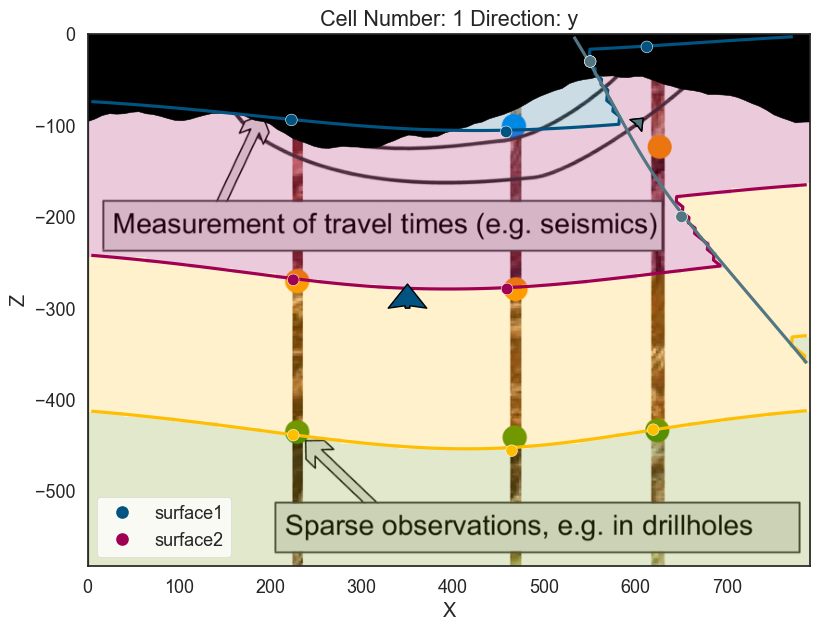

plot_pyvista_to_notebook(p3d.p)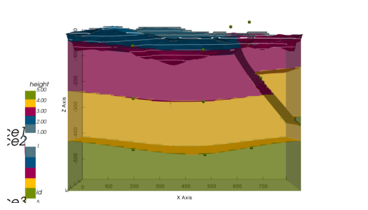

Checkpoint: Next cell will load the model from disk to the necessary state to continue.

geo_model = gp.load_model_pickle(path_to_checkpoint_2)

# Default plotting setting
p2d = gp.plot_2d(geo_model)
ax = p2d.axes[0]
# Reading image
img = mpimg.imread('wells.png')
# Plotting it inplace
ax.imshow(img, origin='upper', alpha=.8, extent = (0, 791, -582,0))
p3d = gp.plot_3d(geo_model, plotter_type='background', show_topography=True)

Part II: Subsurface to GemPy¶

For this notebook we will need some additional packages:

Extra: $ pip install subsurface, pooch, striplog, welly

!pip install subsurface
!pip install pooch
!pip install git+https://github.com/Leguark/striplog.git
!pip install welly
!pip install sklearn

Requirement already satisfied: subsurface in c:\users\legui\appdata\local\programs\python\python39\lib\site-packages (0.2.0)
Requirement already satisfied: numpy in c:\users\legui\appdata\local\programs\python\python39\lib\site-packages (from subsurface) (1.20.1)
Requirement already satisfied: pandas in c:\users\legui\appdata\local\programs\python\python39\lib\site-packages (from subsurface) (1.2.3)
Requirement already satisfied: xarray in c:\users\legui\appdata\local\programs\python\python39\lib\site-packages (from subsurface) (0.17.0)
Requirement already satisfied: python-dateutil>=2.7.3 in c:\users\legui\appdata\local\programs\python\python39\lib\site-packages (from pandas->subsurface) (2.8.1)
Requirement already satisfied: pytz>=2017.3 in c:\users\legui\appdata\local\programs\python\python39\lib\site-packages (from pandas->subsurface) (2021.1)
Requirement already satisfied: setuptools>=40.4 in c:\users\legui\appdata\local\programs\python\python39\lib\site-packages (from xarray->subsurface) (49.2.1)
Requirement already satisfied: six>=1.5 in c:\users\legui\appdata\local\programs\python\python39\lib\site-packages (from python-dateutil>=2.7.3->pandas->subsurface) (1.15.0)

WARNING: You are using pip version 20.2.3; however, version 21.0.1 is available.
You should consider upgrading via the 'c:\users\legui\appdata\local\programs\python\python39\python.exe -m pip install --upgrade pip' command.

Requirement already satisfied: pooch in c:\users\legui\appdata\local\programs\python\python39\lib\site-packages (1.3.0)
Requirement already satisfied: appdirs in c:\users\legui\appdata\local\programs\python\python39\lib\site-packages (from pooch) (1.4.4)
Requirement already satisfied: requests in c:\users\legui\appdata\local\programs\python\python39\lib\site-packages (from pooch) (2.25.1)
Requirement already satisfied: packaging in c:\users\legui\appdata\local\programs\python\python39\lib\site-packages (from pooch) (20.9)
Requirement already satisfied: certifi>=2017.4.17 in c:\users\legui\appdata\local\programs\python\python39\lib\site-packages (from requests->pooch) (2020.12.5)
Requirement already satisfied: chardet<5,>=3.0.2 in c:\users\legui\appdata\local\programs\python\python39\lib\site-packages (from requests->pooch) (4.0.0)
Requirement already satisfied: urllib3<1.27,>=1.21.1 in c:\users\legui\appdata\local\programs\python\python39\lib\site-packages (from requests->pooch) (1.26.4)
Requirement already satisfied: idna<3,>=2.5 in c:\users\legui\appdata\local\programs\python\python39\lib\site-packages (from requests->pooch) (2.10)
Requirement already satisfied: pyparsing>=2.0.2 in c:\users\legui\appdata\local\programs\python\python39\lib\site-packages (from packaging->pooch) (2.4.7)

WARNING: You are using pip version 20.2.3; however, version 21.0.1 is available.
You should consider upgrading via the 'c:\users\legui\appdata\local\programs\python\python39\python.exe -m pip install --upgrade pip' command.

Collecting git+https://github.com/Leguark/striplog.git
  Cloning https://github.com/Leguark/striplog.git to c:\users\legui\appdata\local\temp\pip-req-build-t90fnu3u
Requirement already satisfied (use --upgrade to upgrade): striplog==0.8.5 from git+https://github.com/Leguark/striplog.git in c:\users\legui\appdata\local\programs\python\python39\lib\site-packages
Requirement already satisfied: numpy in c:\users\legui\appdata\local\programs\python\python39\lib\site-packages (from striplog==0.8.5) (1.20.1)
Requirement already satisfied: matplotlib in c:\users\legui\appdata\local\programs\python\python39\lib\site-packages (from striplog==0.8.5) (3.3.4)
Requirement already satisfied: scipy in c:\users\legui\appdata\local\programs\python\python39\lib\site-packages (from striplog==0.8.5) (1.6.2)
Requirement already satisfied: pillow>=6.2.0 in c:\users\legui\appdata\local\programs\python\python39\lib\site-packages (from matplotlib->striplog==0.8.5) (8.1.2)
Requirement already satisfied: cycler>=0.10 in c:\users\legui\appdata\local\programs\python\python39\lib\site-packages (from matplotlib->striplog==0.8.5) (0.10.0)
Requirement already satisfied: pyparsing!=2.0.4,!=2.1.2,!=2.1.6,>=2.0.3 in c:\users\legui\appdata\local\programs\python\python39\lib\site-packages (from matplotlib->striplog==0.8.5) (2.4.7)
Requirement already satisfied: python-dateutil>=2.1 in c:\users\legui\appdata\local\programs\python\python39\lib\site-packages (from matplotlib->striplog==0.8.5) (2.8.1)
Requirement already satisfied: kiwisolver>=1.0.1 in c:\users\legui\appdata\local\programs\python\python39\lib\site-packages (from matplotlib->striplog==0.8.5) (1.3.1)
Requirement already satisfied: six in c:\users\legui\appdata\local\programs\python\python39\lib\site-packages (from cycler>=0.10->matplotlib->striplog==0.8.5) (1.15.0)
Using legacy 'setup.py install' for striplog, since package 'wheel' is not installed.

WARNING: You are using pip version 20.2.3; however, version 21.0.1 is available.
You should consider upgrading via the 'c:\users\legui\appdata\local\programs\python\python39\python.exe -m pip install --upgrade pip' command.

Requirement already satisfied: welly in c:\users\legui\appdata\local\programs\python\python39\lib\site-packages (0.4.9)
Requirement already satisfied: numpy in c:\users\legui\appdata\local\programs\python\python39\lib\site-packages (from welly) (1.20.1)
Requirement already satisfied: scipy in c:\users\legui\appdata\local\programs\python\python39\lib\site-packages (from welly) (1.6.2)
Requirement already satisfied: matplotlib in c:\users\legui\appdata\local\programs\python\python39\lib\site-packages (from welly) (3.3.4)
Requirement already satisfied: lasio in c:\users\legui\appdata\local\programs\python\python39\lib\site-packages (from welly) (0.28)
Requirement already satisfied: striplog in c:\users\legui\appdata\local\programs\python\python39\lib\site-packages (from welly) (0.8.5)
Requirement already satisfied: tqdm in c:\users\legui\appdata\local\programs\python\python39\lib\site-packages (from welly) (4.59.0)
Requirement already satisfied: pillow>=6.2.0 in c:\users\legui\appdata\local\programs\python\python39\lib\site-packages (from matplotlib->welly) (8.1.2)
Requirement already satisfied: cycler>=0.10 in c:\users\legui\appdata\local\programs\python\python39\lib\site-packages (from matplotlib->welly) (0.10.0)
Requirement already satisfied: kiwisolver>=1.0.1 in c:\users\legui\appdata\local\programs\python\python39\lib\site-packages (from matplotlib->welly) (1.3.1)
Requirement already satisfied: python-dateutil>=2.1 in c:\users\legui\appdata\local\programs\python\python39\lib\site-packages (from matplotlib->welly) (2.8.1)
Requirement already satisfied: pyparsing!=2.0.4,!=2.1.2,!=2.1.6,>=2.0.3 in c:\users\legui\appdata\local\programs\python\python39\lib\site-packages (from matplotlib->welly) (2.4.7)
Requirement already satisfied: six in c:\users\legui\appdata\local\programs\python\python39\lib\site-packages (from cycler>=0.10->matplotlib->welly) (1.15.0)

WARNING: You are using pip version 20.2.3; however, version 21.0.1 is available.
You should consider upgrading via the 'c:\users\legui\appdata\local\programs\python\python39\python.exe -m pip install --upgrade pip' command.

Requirement already satisfied: sklearn in c:\users\legui\appdata\local\programs\python\python39\lib\site-packages (0.0)
Requirement already satisfied: scikit-learn in c:\users\legui\appdata\local\programs\python\python39\lib\site-packages (from sklearn) (0.24.1)
Requirement already satisfied: threadpoolctl>=2.0.0 in c:\users\legui\appdata\local\programs\python\python39\lib\site-packages (from scikit-learn->sklearn) (2.1.0)
Requirement already satisfied: scipy>=0.19.1 in c:\users\legui\appdata\local\programs\python\python39\lib\site-packages (from scikit-learn->sklearn) (1.6.2)
Requirement already satisfied: joblib>=0.11 in c:\users\legui\appdata\local\programs\python\python39\lib\site-packages (from scikit-learn->sklearn) (1.0.1)
Requirement already satisfied: numpy>=1.13.3 in c:\users\legui\appdata\local\programs\python\python39\lib\site-packages (from scikit-learn->sklearn) (1.20.1)

WARNING: You are using pip version 20.2.3; however, version 21.0.1 is available.
You should consider upgrading via the 'c:\users\legui\appdata\local\programs\python\python39\python.exe -m pip install --upgrade pip' command.

Subsurface: Centralizing data management for the GeoScientific Stack¶

Subsurface is a package in development aiming to unify at a low level the data structures used from multilpe packages in geoscience for Python. It heavily relies on xarray to store data.

Besides the data structures themselves subsurface provides custom logic to read - and in the future write - to 3rd party formats outside the Python ecosystem. In this notebook we are going to use subsurface to import borehole data from csv files:

import pooch
from striplog import Component
import pandas as pd
import numpy as np

import subsurface as sb
from subsurface.reader import ReaderFilesHelper
from subsurface.reader.wells import read_collar, read_lith, read_survey, WellyToSubsurfaceHelper, welly_to_subsurface

We use pooch to download the dataset into a temp file:

url = "https://raw.githubusercontent.com/softwareunderground/subsurface/main/tests/data/borehole/kim_ready.csv"
known_hash = "efa90898bb435daa15912ca6f3e08cd3285311923a36dbc697d2aafebbafa25f"

# Your code here:
raw_borehole_data_csv = pooch.retrieve(url, known_hash)

Now we can use subsurface function to help us reading csv files into pandas dataframes that the package can understand. Since the combination of styles data is provided can highly vary from project to project, subsurface provides some helpers functions to parse different combination of .csv

reading_collars = ReaderFilesHelper(
        file_or_buffer=raw_borehole_data_csv,
        index_col="name",
        usecols=['x', 'y', 'altitude', "name"]
    )

reading_collars

ReaderFilesHelper(file_or_buffer='C:\\Users\\legui\\AppData\\Local\\pooch\\pooch\\Cache\\7c2d6aa7551f31216f7236d3f9fb70a6-kim_ready.csv', usecols=['x', 'y', 'altitude', 'name'], col_names=None, drop_cols=None, format='.csv', index_map=None, columns_map=None, additional_reader_kwargs={}, file_or_buffer_type=<class 'str'>, index_col='name', header='infer')

from dataclasses import asdict
asdict(reading_collars)

{'file_or_buffer': 'C:\\Users\\legui\\AppData\\Local\\pooch\\pooch\\Cache\\7c2d6aa7551f31216f7236d3f9fb70a6-kim_ready.csv',
 'usecols': ['x', 'y', 'altitude', 'name'],
 'col_names': None,
 'drop_cols': None,
 'format': '.csv',
 'index_map': None,
 'columns_map': None,
 'additional_reader_kwargs': {},
 'file_or_buffer_type': str,
 'index_col': 'name',
 'header': 'infer'}

collar = read_collar(reading_collars)

collar

# Your code here:
survey = read_survey(
    ReaderFilesHelper(
        file_or_buffer=raw_borehole_data_csv,
        index_col="name",
        usecols=["name", "md"]
    )
)

survey

# Your code here:
lith = read_lith(
    ReaderFilesHelper(
        file_or_buffer=raw_borehole_data_csv,
        usecols=['name', 'top', 'base', 'formation'],
        columns_map={'top': 'top',
                     'base': 'base',
                     'formation': 'component lith',
                     }
    )
)

lith

Welly¶

Welly is a family of classes to facilitate the loading, processing, and analysis of subsurface wells and well data, such as striplogs, formation tops, well log curves, and synthetic seismograms.

We are using welly to convert pandas data frames into classes to manipulate well data. The final goal is to extract 3D coordinates and properties for multiple wells.

The class WellyToSubsurfaceHelper contains the methods to create a welly project and export it to a subsurface data class.

wts = sb.reader.wells.WellyToSubsurfaceHelper(collar_df=collar, survey_df=survey, lith_df=lith)

The following striplog failed being processed:  []

In the field p is stored a welly project (https://github.com/agile-geoscience/welly/blob/master/tutorial/04_Project.ipynb)and we can use it to explore and visualize properties of each well.

wts.p

stripLog = wts.p[0].data['lith']
stripLog

Striplog(10 Intervals, start=0.0, stop=4594.951477330001)

stripLog.plot()
plt.gcf()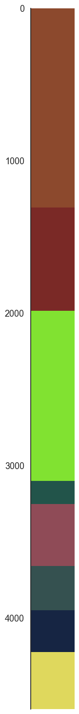

welly_well = wts.p[0].data["lith_log"]
welly_well

Welly to Subsurface¶

Welly is a very powerful tool to inspect well data but it was not design for 3D. However they have a method to export XYZ coordinates of each of the well that we can take advanatage of to create a subsurface.UnstructuredData object. This object is one of the core data class of subsurface and we will use it from now on to keep working in 3D.

formations = ["topo", "etchegoin", "macoma", "chanac", "mclure",
              "santa_margarita", "fruitvale",
              "round_mountain", "olcese", "freeman_jewett", "vedder", "eocene",
              "cretaceous",
              "basement", "null"]

unstruct = sb.reader.wells.welly_to_subsurface(wts, table=[Component({'lith': l}) for l in formations])
unstruct.data

At each core UstructuredData is a wrapper of a xarray.Dataset. Although slightly flexible, any UnstructuredData will contain 4 xarray.DataArray objects containing vertex, cells, cell attributes and vertex attibutes. This is the minimum amount of information necessary to work in 3D.

From an UnstructuredData we can construct elements. elements are a higher level construct and includes the definion of type of geometric representation - e.g. points, lines, surfaces, etc. For the case of borehole we will use LineSets. elements have a very close relation to vtk data structures what enables easily to plot the data using pyvista

element = sb.LineSet(unstruct)
pyvista_mesh = sb.visualization.to_pyvista_line(element, radius=50)

# Plot default LITH
interactive_plot =sb.visualization.pv_plot([pyvista_mesh], background_plotter=True)

plot_pyvista_to_notebook(interactive_plot)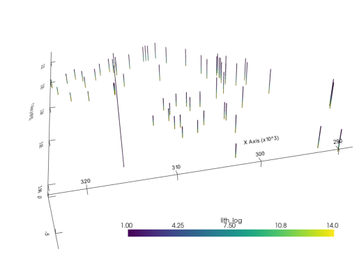

Finding the boreholes bases¶

GemPy interpolates the bottom of a unit, therefore we need to be able to extract those points to be able tointerpolate them. xarray, pandas and numpy are using the same type of memory representation what makes possible to use the same or at least similar methods to manipulate the data to our will.

Lets find the base points of each well:

# Creating references to the xarray.DataArray
cells_attr = unstruct.data.cell_attrs
cells = unstruct.data.cells
vertex = unstruct.data.vertex

# Find vertex points at the boundary of two units
# Marking each vertex
bool_prop_change = cells_attr.values[1:] != cells_attr.values[:-1]
# Getting the index of the vertex
args_prop_change = np.where(bool_prop_change)[0]
# Getting the attr values at those points 
vals_prop_change = cells_attr[args_prop_change]
vals_prop_change.to_pandas()

# Getting the vertex values at those points
vertex_args_prop_change = cells[args_prop_change, 1]
interface_points = vertex[vertex_args_prop_change]
interface_points

# Creating a new UnstructuredData
interf_us= sb.UnstructuredData.from_array(vertex=interface_points.values, cells="points",
                                          cells_attr=vals_prop_change.to_pandas())
interf_us

<xarray.Dataset>
Dimensions:       (XYZ: 3, cell: 595, cell_attr: 1, nodes: 1, points: 595, vertex_attr: 0)
Coordinates:
  * points        (points) int64 0 1 2 3 4 5 6 7 ... 588 589 590 591 592 593 594
  * XYZ           (XYZ) <U1 'X' 'Y' 'Z'
  * cell_attr     (cell_attr) object 'lith_log'
  * vertex_attr   (vertex_attr) int64 
    cell_         (cell) int64 0 1 2 3 4 5 6 7 ... 588 589 590 591 592 593 594
Dimensions without coordinates: cell, nodes
Data variables:
    vertex        (points, XYZ) float64 2.753e+05 3.947e+06 ... -2.907e+03
    cells         (cell, nodes) int32 0 1 2 3 4 5 6 ... 589 590 591 592 593 594
    cell_attrs    (cell, cell_attr) int32 1 2 3 5 8 9 12 13 ... 3 4 6 9 10 11 13
    vertex_attrs  (points, vertex_attr) float64

This new UnstructuredData object instead containing data that represent lines, contain point data at the bottom of each unit. We can plot it very similar as before:

element = sb.PointSet(interf_us)
pyvista_mesh = sb.visualization.to_pyvista_points(element)
interactive_plot.add_mesh(pyvista_mesh)

(vtkmodules.vtkRenderingOpenGL2.vtkOpenGLActor)0000028F136BBE80

plot_pyvista_to_notebook(interactive_plot)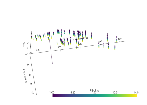

GemPy: Initialize model¶

Regular grid: default grid mainly for general visualization
Custom grid: GemPy's wrapper to interpolate on a user grid
Topography: Topographic data use to be of high density. Treating it as an independent grid allow for high resolution geological maps
Sections: If we predefine the section 2D grid we can directly interpolate at those locations for perfect, high resolution estimations
Center grids: Half sphere grids around a given point at surface. This are specially tuned for geophysical forward computations

import gempy as gp
extent= [275619, 323824, 3914125, 3961793, -3972.6, 313.922]

# Your code here:
geo_model = gp.create_model("getting started")
geo_model.set_regular_grid(extent=extent, resolution=[50,50,50])

Active grids: ['regular']

Grid Object. Values: 
array([[ 2.76101050e+05,  3.91460168e+06, -3.92973478e+03],
       [ 2.76101050e+05,  3.91460168e+06, -3.84400434e+03],
       [ 2.76101050e+05,  3.91460168e+06, -3.75827390e+03],
       ...,
       [ 3.23341950e+05,  3.96131632e+06,  9.95959000e+01],
       [ 3.23341950e+05,  3.96131632e+06,  1.85326340e+02],
       [ 3.23341950e+05,  3.96131632e+06,  2.71056780e+02]])

GemPy core code is written in Python. However for efficiency and gradient based machine learning most of heavy computations happen in optimize compile code, either C or CUDA for GPU.

gp.set_interpolator(geo_model, theano_optimizer='fast_compile', verbose=[])

Setting kriging parameters to their default values.
Compiling theano function...
Level of Optimization:  fast_compile
Device:  cpu
Precision:  float64
Number of faults:  0
Compilation Done!
Kriging values: 
                            values
range                67928.893115
$C_o$            109865107.615631
drift equations               [3]

<gempy.core.interpolator.InterpolatorModel at 0x28f1378ce50>

Making a model step by step.¶

The temptation at this point is to bring all the points into gempy and just interpolate. However, often that strategy results in ill posed problems due to noise or irregularities in the data. gempy has been design to being able to iterate rapidly and therefore a much better workflow use to be creating the model step by step.

To do that, lets define a function that we can pass the name of the formation and get the assotiated vertex. Grab from the interf_us the XYZ coordinates of the first layer:

def get_interface_coord_from_surfaces(surface_names: list, verbose=False):
    
    df = pd.DataFrame(columns=["X", "Y", "Z", "surface"])
    
    for e, surface_name in enumerate(surface_names):
        # The properties in subsurface start at 1
        val_property = formations.index(surface_name) + 1
        # Find the cells with the surface id
        args_from_first_surface = np.where(vals_prop_change == val_property)[0]    
        if verbose: print(args_from_first_surface)
        # Find the vertex
        points_from_first_surface = interface_points[args_from_first_surface]
        if verbose: print(points_from_first_surface)
        
        # xarray.DataArray to pandas.DataFrame
        surface_pandas = points_from_first_surface.to_pandas()
        
        # Add formation column
        surface_pandas["surface"] = surface_name
        df = df.append(surface_pandas)
    
    return df.reset_index()

Surfaces¶

GemPy is a surface based interpolator. This means that all the input data we add has to be refereed to a surface. The surfaces always mark the bottom of a unit.

This is a list with the formations names for this data set.

formations

['topo',
 'etchegoin',
 'macoma',
 'chanac',
 'mclure',
 'santa_margarita',
 'fruitvale',
 'round_mountain',
 'olcese',
 'freeman_jewett',
 'vedder',
 'eocene',
 'cretaceous',
 'basement',
 'null']

Lets add the first two (remember we always need a basement defined).

geo_model.add_surfaces(formations[:2])

Using the function defined above we just extract the surface points for topo:

gempy_surface_points = get_interface_coord_from_surfaces(["topo"])
gempy_surface_points

And we can set them into the gempy model:

geo_model.set_surface_points(gempy_surface_points, update_surfaces=False)
geo_model.update_to_interpolator()

True

g2d = gp.plot_2d(geo_model)

g2d.fig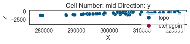

The minimum amount of input data to interpolate anything in gempy is:

a) 2 surface points per surface

b) One orientation per series.

Lets add an orientation:

geo_model.add_orientations(X=300000, Y=3930000, Z=0, surface="topo", pole_vector=(0,0,1))

At current state (gempy 2.2), the data classes are:

gempy.SurfacePoints
gempy.Orientations
gempy.Surfaces
gempy.Stack (combination of gempy.Series and gempy.Faults)
gempy.Grid
gempy.AdditionalData
gempy.Solutions

Today we will look into details only some of these classes but what is important to notice is that you can access these objects as follows:

geo_model.additional_data

gp.compute_model(geo_model)


Lithology ids 
  [2. 2. 2. ... 2. 2. 2.]

g3d = gp.plot_3d(geo_model, plotter_type="background")

g3d.p.add_mesh(pyvista_mesh)

(vtkmodules.vtkRenderingOpenGL2.vtkOpenGLActor)0000028F7BBC5040

plot_pyvista_to_notebook(g3d.p)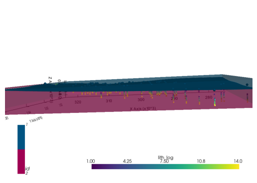

Second layer¶

geo_model.add_surfaces(formations[2])

gempy_surface_points = get_interface_coord_from_surfaces(formations[:2])
geo_model.set_surface_points(gempy_surface_points, update_surfaces=False)
geo_model.update_to_interpolator()

True

gp.compute_model(geo_model)


Lithology ids 
  [1. 1. 1. ... 1. 1. 1.]

live_plot = gp.plot_3d(geo_model, plotter_type="background", show_results=True)

plot_pyvista_to_notebook(live_plot.p)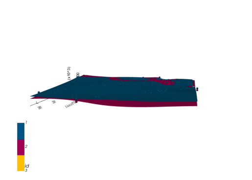

live_plot.toggle_live_updating()

True

Trying to fix the model: Multiple Geo. Features/Series¶

geo_model.add_features("Formations")

geo_model.map_stack_to_surfaces({"Form1": ["etchegoin", "macoma"]}, set_series=False)

geo_model.add_orientations(X=300000, Y=3930000, Z=0, surface="etchegoin", pole_vector=(0,0,1), idx=1)

gp.compute_model(geo_model)


Lithology ids 
  [3. 3. 3. ... 3. 3. 2.]

h3d = gp.plot_3d(geo_model, plotter_type="background", show_lith=False, ve=5)

plot_pyvista_to_notebook(h3d.p)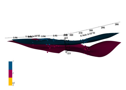

Last layers for today¶

geo_model.add_surfaces(formations[3:5])

f_last = formations[:4]
f_last

['topo', 'etchegoin', 'macoma', 'chanac']

gempy_surface_points = get_interface_coord_from_surfaces(f_last)
geo_model.set_surface_points(gempy_surface_points, update_surfaces=False)
geo_model.update_to_interpolator()

True

gp.compute_model(geo_model)


Lithology ids 
  [2. 2. 2. ... 2. 2. 2.]

p3d_4 = gp.plot_3d(geo_model, plotter_type="background", show_lith=False, ve=5)

plot_pyvista_to_notebook(p3d_4.p)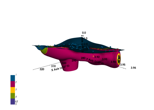

geo_model.add_orientations(X=321687.059770, Y=3.945955e+06, Z=0, surface="etchegoin", pole_vector=(0,0,1), idx=1)
gp.compute_model(geo_model)
p3d_4.plot_surfaces()

{'topo': (vtkmodules.vtkRenderingOpenGL2.vtkOpenGLActor)000001F502C045E0,
 'etchegoin': (vtkmodules.vtkRenderingOpenGL2.vtkOpenGLActor)000001F502CA5FA0,
 'macoma': (vtkmodules.vtkRenderingOpenGL2.vtkOpenGLActor)000001F503552DC0,
 'chanac': (vtkmodules.vtkRenderingOpenGL2.vtkOpenGLActor)000001F55E62FB80}

geo_model.add_orientations(X=277278.652995, Y=3.929298e+06, Z=0, surface="etchegoin", pole_vector=(0,0,1), idx=2)
gp.compute_model(geo_model)
p3d_4.plot_surfaces()

{'topo': (vtkmodules.vtkRenderingOpenGL2.vtkOpenGLActor)000001F502CB29A0,
 'etchegoin': (vtkmodules.vtkRenderingOpenGL2.vtkOpenGLActor)000001F5035590A0,
 'macoma': (vtkmodules.vtkRenderingOpenGL2.vtkOpenGLActor)000001F55E4C6CA0,
 'chanac': (vtkmodules.vtkRenderingOpenGL2.vtkOpenGLActor)000001F55E62F160}

Adding many more orientations¶

# find neighbours
neighbours = gp.select_nearest_surfaces_points(geo_model, geo_model._surface_points.df, 2)

# calculate all fault orientations
new_ori = gp.set_orientation_from_neighbours_all(geo_model, neighbours)
new_ori.df.head()

gp.compute_model(geo_model)


Lithology ids 
  [5.         5.         5.         ... 2.00000078 2.         2.        ]

p3d_4.plot_orientations()
p3d_4.plot_surfaces()

{'topo': (vtkmodules.vtkRenderingOpenGL2.vtkOpenGLActor)000001F559AB40A0,
 'etchegoin': (vtkmodules.vtkRenderingOpenGL2.vtkOpenGLActor)000001F55E62FEE0,
 'macoma': (vtkmodules.vtkRenderingOpenGL2.vtkOpenGLActor)000001F55E62F520,
 'chanac': (vtkmodules.vtkRenderingOpenGL2.vtkOpenGLActor)000001F50354FFA0}

p3d_4.p.add_mesh(pyvista_mesh)

(vtkmodules.vtkRenderingOpenGL2.vtkOpenGLActor)000001F502CA5FA0

plot_pyvista_to_notebook(p3d_4.p)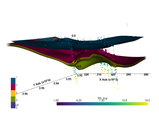

Thank you for your attention¶

Extra Resources¶

Page: https://www.gempy.org/

Paper: https://www.gempy.org/theory

Gitub: https://github.com/cgre-aachen/gempy

Further training and collaborations¶

https://www.terranigma-solutions.com/

T21 - GemPy

t21_gempy.ipynb

Transform 2021: GemPy Workshop¶

Table of Content¶

Installation¶

Part I: Your first model (refresher)¶

Initializing the model... But first a word about Grids:¶

Creating figure:¶

Add model section¶

Loading cross-section image:¶

Building the model¶

Surfaces¶

Intermission: GemPy data classes¶

Adding more layers¶

Layer 2¶

Layer 3¶

Intermission: GemPy data structures: Surfaces Points, Orientations and surfaces¶

Unconformities and Faults:¶

Erosion¶

Onlap¶

Fault¶

Additional features:¶

Topography¶

Part II: Subsurface to GemPy¶

Subsurface: Centralizing data management for the GeoScientific Stack¶

Welly¶

Welly to Subsurface¶

Finding the boreholes bases¶

GemPy: Initialize model¶

Making a model step by step.¶

Surfaces¶

Second layer¶

Trying to fix the model: Multiple Geo. Features/Series¶

Last layers for today¶

Adding many more orientations¶

Thank you for your attention¶

Extra Resources¶

Further training and collaborations¶