Modelling.ipynb
This notebook covers the modelling techniques used for getting optimal prediction results.
Data Cleaning and Preparation
This involves the necessary steps and processing to get both the train and test datasets in an acceptable form for the machine learnning algorithm:
- Creating validation data sets
- Selecting interested logs
- Resolving missing values
- Encoding categorical variables
- Data augmentation
from google.colab import drive
drive.mount('/content/drive', force_remount=True)
Mounted at /content/drive
cd /content/drive/MyDrive/TRANSFORM-2021/content/drive/MyDrive/TRANSFORM-2021
import numpy as np
import random
import pandas as pd
import xgboost as xgb
from sklearn.model_selection import StratifiedKFold
from sklearn.metrics import accuracy_score, f1_score
traindata = pd.read_csv('./data/train.csv', sep=';')
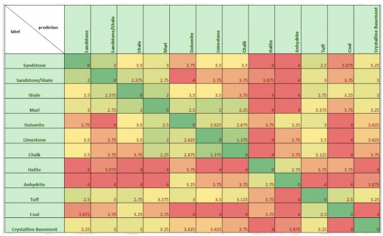
testdata = pd.read_csv('./data/leaderboard_test_features.csv.txt', sep=';')A = np.load('./data/penalty_matrix.npy') # panlty matrix used for scoringAarray([[0. , 2. , 3.5 , 3. , 3.75 , 3.5 , 3.5 , 4. , 4. ,
2.5 , 3.875, 3.25 ],
[2. , 0. , 2.375, 2.75 , 4. , 3.75 , 3.75 , 3.875, 4. ,
3. , 3.75 , 3. ],
[3.5 , 2.375, 0. , 2. , 3.5 , 3.5 , 3.75 , 4. , 4. ,
2.75 , 3.25 , 3. ],
[3. , 2.75 , 2. , 0. , 2.5 , 2. , 2.25 , 4. , 4. ,
3.375, 3.75 , 3.25 ],
[3.75 , 4. , 3.5 , 2.5 , 0. , 2.625, 2.875, 3.75 , 3.25 ,
3. , 4. , 3.625],
[3.5 , 3.75 , 3.5 , 2. , 2.625, 0. , 1.375, 4. , 3.75 ,
3.5 , 4. , 3.625],
[3.5 , 3.75 , 3.75 , 2.25 , 2.875, 1.375, 0. , 4. , 3.75 ,
3.125, 4. , 3.75 ],
[4. , 3.875, 4. , 4. , 3.75 , 4. , 4. , 0. , 2.75 ,
3.75 , 3.75 , 4. ],
[4. , 4. , 4. , 4. , 3.25 , 3.75 , 3.75 , 2.75 , 0. ,
4. , 4. , 3.875],
[2.5 , 3. , 2.75 , 3.375, 3. , 3.5 , 3.125, 3.75 , 4. ,
0. , 2.5 , 3.25 ],
[3.875, 3.75 , 3.25 , 3.75 , 4. , 4. , 4. , 3.75 , 4. ,
2.5 , 0. , 4. ],
[3.25 , 3. , 3. , 3.25 , 3.625, 3.625, 3.75 , 4. , 3.875,
3.25 , 4. , 0. ]])Scoring matrix for petrophysical interpretation

def score(y_true, y_pred):

    '''
    custom metric used for evaluation
    args:
      y_true: actual prediction
      y_pred: predictions made
    '''

    S = 0.0
    y_true = y_true.astype(int)
    y_pred = y_pred.astype(int)
    for i in range(0, y_true.shape[0]):
        S -= A[y_true[i], y_pred[i]]
    return S/y_true.shape[0]
Creating Validation Sets
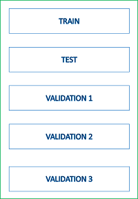
Validation sets are created to properly evaluate changes made on the machine learning model. This is important to prevent overfitting the open test data since the blind test is used as the final determiner. So it is important to build ML models that will generalise better on unseen wells. Having no idea how the blind wells would come (geospatial distribution, logs presence), there was no specific guide in selecting train wells, so wells were randomly selected from the train to create two validation sets (each comprising of 10 wells).
train_wells = traindata.WELL.unique()print(f'Initial total number of train wells: {len(train_wells)}')Initial total number of train wells: 98
np.random.seed(40)valid1 = random.sample(list(train_wells), 10) #randomly sample 10 well names from train dataQC to remove valid1 wells from train wells to prevent having same well(s) in the second validation data
train_wells = [well for well in train_wells if not well in valid1]
print(f'Number of wells left: {len(train_wells)}')
Number of wells left: 88
valid2 = random.sample(list(train_wells), 10)

train_wells = [well for well in train_wells if not well in valid2]
print(f'Number of wells left: {len(train_wells)}')
Number of wells left: 78
print(len(valid1), len(valid2))10 10
validation_wells = set(valid1 + valid2)
print(len(validation_wells))
20
Let's proceed to getting the validation data from the train data set and dropping them to prevent any form of data leakage.
def create_validation_set(train, wells):

    '''
    Function to validation sets from the full train data using well names
    '''

    validation = pd.DataFrame(columns=list(train.columns))

    for well in wells:
        welldata = train.loc[train.WELL == well]
        validation = pd.concat((welldata, validation))

    return validation
# using function to get data for validation wells
validation1 = create_validation_set(traindata, valid1)
validation2 = create_validation_set(traindata, valid2)# total validation data
validation = pd.concat((validation1, validation2))validation.shape, validation1.shape, validation2.shape((232527, 29), (123486, 29), (109041, 29))# dropping validation data from train data
new_train = pd.concat([traindata, validation, validation]).drop_duplicates(keep=False)
print(f'Previous train data shape: {traindata.shape}')
print(f'New train data shape: {new_train.shape}')Previous train data shape: (1170511, 29)
New train data shape: (937984, 29)
# QC to ensure there are no data leakage

previous_rows = traindata.shape[0]
new_train_rows = new_train.shape[0]
validation_rows = validation.shape[0]

print(f'Number of previous train data rows: {previous_rows}')
print(f'Validation + validation rows: {validation_rows+new_train_rows}')
Number of previous train data rows: 1170511
Validation + validation rows: 1170511
# to confirm we still have all samples of the labels in the train data set

new_train.FORCE_2020_LITHOFACIES_LITHOLOGY.value_counts()
65000 573405
30000 136783
65030 120134
70000 45086
80000 26950
99000 11381
70032 10401
88000 8213
90000 3107
74000 1336
86000 1085
93000 103
Name: FORCE_2020_LITHOFACIES_LITHOLOGY, dtype: int64Now we can proceed to other preparation procedures.
Logs were selected based on user's desire to use them for training. The confidence logs was dropped as this was absent in the test logs as the ML models need the same set of wells used for training in making predictions on the test wells. Other absent logs and logs with low percentage of values from the combined test data are also dropped. This has previously been visualized in the EDA notebook. A cut off of 30% may be selected as criteria for dropping the logs. Let's take a look at that!
print(f'Percentage of values in test logs:')
100 - testdata.isna().sum()/testdata.shape[0]*100
Percentage of values in test logs:
WELL         100.000000
DEPTH_MD     100.000000
X_LOC         99.956867
Y_LOC         99.956867
Z_LOC         99.956867
GROUP        100.000000
FORMATION     94.828418
CALI          95.873116
RSHA          28.582603
RMED          99.570863
RDEP          99.956867
RHOB          87.601070
GR           100.000000
SGR            0.000000
NPHI          76.062609
PEF           82.978521
DTC           99.398330
SP            48.708932
BS            48.955302
ROP           49.943708
DTS           31.596801
DCAL           9.880397
DRHO          81.555130
MUDWEIGHT     14.818037
RMIC           8.272776
ROPA          40.786338
RXO           21.820947
dtype: float64
For better and faster processing, the train, validation and test data sets will be concatenated and processed together as we need these data sets to be in the same formats to get good predictions out of the ML model. But let's have it in mind that the RSHA, SGR, DCAL, MUDWEIGHT, RMIC and RXO will be dropped from the wells. Let's proceed.
Let's extract the data sets indices that will be used for splitting the features and targets into their respective datasets after prepration is complete. We will also be extracting the train target
ntrain = new_train.shape[0]
ntest = testdata.shape[0]
nvalid1 = validation1.shape[0]
nvalid2 = validation2.shape[0]
nvalid3 = validation.shape[0]

df = pd.concat((new_train, testdata, validation1, validation2, validation)).reset_index(drop=True)
So the combined dataframe for preparation

df.shape(1539824, 29)The procedure below is used to extract data needed for the augmentation procedure to be performed after every other preparation has been done
#making a copy of the dataframes

train = new_train.copy()
test = testdata.copy()
valid1 = validation1.copy()
valid2 = validation2.copy()
valid = validation.copy()
# extracting the data sets well names and depth values needed for augmentation
train_well = train.WELL.values
train_depth = train.DEPTH_MD.values
test_well = test.WELL.values
test_depth = test.DEPTH_MD.values
valid1_well = valid1.WELL.values
valid1_depth = valid1.DEPTH_MD.values
valid2_well = valid2.WELL.values
valid2_depth = valid2.DEPTH_MD.values
valid_well = valid.WELL.values
valid_depth = valid.DEPTH_MD.valuesNow let's extract the data sets labels and prepare them for training and validation performance check.
lithology = train['FORCE_2020_LITHOFACIES_LITHOLOGY']
valid1_lithology = valid1['FORCE_2020_LITHOFACIES_LITHOLOGY']
valid2_lithology = valid2['FORCE_2020_LITHOFACIES_LITHOLOGY']
valid_lithology = valid['FORCE_2020_LITHOFACIES_LITHOLOGY']

lithology_numbers = {30000: 0,
                 65030: 1,
                 65000: 2,
                 80000: 3,
                 74000: 4,
                 70000: 5,
                 70032: 6,
                 88000: 7,
                 86000: 8,
                 99000: 9,
                 90000: 10,
                 93000: 11}

lithology = lithology.map(lithology_numbers)
valid1_lithology = valid1_lithology.map(lithology_numbers)
valid2_lithology = valid2_lithology.map(lithology_numbers)
valid_lithology = valid_lithology.map(lithology_numbers)
print(f'dataframe shapes before dropping columns: {df.shape}')
def drop_columns(data, *args):
'''
function used to drop columns.
args::
data: dataframe to be operated on
*args: a list of columns to be dropped from the dataframe
return: returns a dataframe with the columns dropped
'''
columns = []
for _ in args:
columns.append(_)
data = data.drop(columns, axis=1)
return data
columns_dropped = ['RSHA', 'SGR', 'DCAL', 'MUDWEIGHT', 'RMIC', 'RXO'] #columns to be dropped
df = drop_columns(df, *columns_dropped)
print(f'shape of dataframe after dropping columns {df.shape}')dataframe shapes before dropping columns: (1539824, 29)
shape of dataframe after dropping columns (1539824, 23)
Data Encoding
The categorical logs/columns in the data set need to be encoded for use by the ML algorithm. From the data visualization, we saw the high dimensionality of the logs (especially the FORMATION log with 69 distinct values), so label encoding will be applied instead of one hot encoding these features to prevent high dimensionality of the data.
df['GROUP_encoded'] = df['GROUP'].astype('category')
df['GROUP_encoded'] = df['GROUP_encoded'].cat.codes

df['FORMATION_encoded'] = df['FORMATION'].astype('category')
df['FORMATION_encoded'] = df['FORMATION_encoded'].cat.codes

df['WELL_encoded'] = df['WELL'].astype('category')
df['WELL_encoded'] = df['WELL_encoded'].cat.codes

print(f'shape of dataframe after label encoding columns {df.shape}')
shape of dataframe after label encoding columns (1539824, 26)
# dropping the previous columns after encoding

df = df.drop(['WELL', 'GROUP', 'FORMATION'], axis=1)
Filling Missing Values
Some fractions of missing values still exist in present logs, how do we resolve that? While we can use a mean of values in a window to solve this, backward or forward fill, we could also decide to fill up all missing values with a distinct value different from other values. This way, the ML algorithm used (in this case a gradient tree algorithm) can differentiate this better. From validation, this improved result better. -9999 is used, and since this is a classification problem as opposed to a regression where we predict actual lithology values, outlier effect is not observed in the output.
df = df.fillna(-9999)df.isna().sum()/df.shape[0]*100DEPTH_MD 0.0
X_LOC 0.0
Y_LOC 0.0
Z_LOC 0.0
CALI 0.0
RMED 0.0
RDEP 0.0
RHOB 0.0
GR 0.0
NPHI 0.0
PEF 0.0
DTC 0.0
SP 0.0
BS 0.0
ROP 0.0
DTS 0.0
DRHO 0.0
ROPA 0.0
FORCE_2020_LITHOFACIES_LITHOLOGY 0.0
FORCE_2020_LITHOFACIES_CONFIDENCE 0.0
GROUP_encoded 0.0
FORMATION_encoded 0.0
WELL_encoded 0.0
dtype: float64Now that we've completed the majority of the preparation, let's split back our concatenated dataframe into their validation sets, train and test set
data = df.copy()   #making a copy of the preparaed dataframe to work with
data.shape
(1539824, 23)Remember the shape of the concatenated dataframe;

using the data sets indices will be used for slicing out their corresponding features
train = data[:ntrain].copy()
train.drop(['FORCE_2020_LITHOFACIES_LITHOLOGY'], axis=1, inplace=True)

test = data[ntrain:(ntest+ntrain)].copy()
test.drop(['FORCE_2020_LITHOFACIES_LITHOLOGY'], axis=1, inplace=True)
test = test.reset_index(drop=True)

valid1 = data[(ntest+ntrain):(ntest+ntrain+nvalid1)].copy()
valid1.drop(['FORCE_2020_LITHOFACIES_LITHOLOGY'], axis=1, inplace=True)
valid1 = valid1.reset_index(drop=True)

valid2 = data[(ntest+ntrain+nvalid1):(ntest+ntrain+nvalid1+nvalid2)].copy()
valid2.drop(['FORCE_2020_LITHOFACIES_LITHOLOGY'], axis=1, inplace=True)
valid2 = valid2.reset_index(drop=True)

valid = data[(ntest+ntrain+nvalid1+nvalid2):].copy()
valid.drop(['FORCE_2020_LITHOFACIES_LITHOLOGY'], axis=1, inplace=True)
valid = valid.reset_index(drop=True)
# checking shapes of sliced data sets for QC
train.shape, test.shape, valid1.shape, valid2.shape, valid.shape((937984, 22), (136786, 22), (123486, 22), (109041, 22), (232527, 22))Data Augmentation
The data augmentation technique is extracted from the ISPL team code for the 2016 SEG ML competition : https://github.com/seg/2016-ml-contest/tree/master/ispl . The technique was based on the assumption that "facies do not abrutly change from a given depth layer to the next one". This was implemented by aggregating features at neighbouring depths and computing the feature spatial gradient.
# Feature windows concatenation function
def augment_features_window(X, N_neig):

    # Parameters
    N_row = X.shape[0]
    N_feat = X.shape[1]

    # Zero padding
    X = np.vstack((np.zeros((N_neig, N_feat)), X, (np.zeros((N_neig, N_feat)))))

    # Loop over windows
    X_aug = np.zeros((N_row, N_feat*(2*N_neig+1)))
    for r in np.arange(N_row)+N_neig:
        this_row = []
        for c in np.arange(-N_neig,N_neig+1):
            this_row = np.hstack((this_row, X[r+c]))
        X_aug[r-N_neig] = this_row

    return X_aug

# Feature gradient computation function
def augment_features_gradient(X, depth):

    # Compute features gradient
    d_diff = np.diff(depth).reshape((-1, 1))
    d_diff[d_diff==0] = 0.001
    X_diff = np.diff(X, axis=0)
    X_grad = X_diff / d_diff

    # Compensate for last missing value
    X_grad = np.concatenate((X_grad, np.zeros((1, X_grad.shape[1]))))

    return X_grad

# Feature augmentation function
def augment_features(X, well, depth, N_neig=1):

    # Augment features
    X_aug = np.zeros((X.shape[0], X.shape[1]*(N_neig*2+2)))
    for w in np.unique(well):
        w_idx = np.where(well == w)[0]
        X_aug_win = augment_features_window(X[w_idx, :], N_neig)
        X_aug_grad = augment_features_gradient(X[w_idx, :], depth[w_idx])
        X_aug[w_idx, :] = np.concatenate((X_aug_win, X_aug_grad), axis=1)

    return X_aug
print(f'Shape of datasets before augmentation {train.shape, test.shape, valid1.shape, valid2.shape, valid.shape}')
aug_train = augment_features(train.values, train_well, train_depth)
aug_test = augment_features(test.values, test_well, test_depth)
aug_valid1 = augment_features(valid1.values, valid1_well, valid1_depth)
aug_valid2 = augment_features(valid2.values, valid2_well, valid2_depth)
aug_valid = augment_features(valid.values, valid_well, valid_depth)
print(f'Shape of datasets after augmentation {aug_train.shape, aug_test.shape, aug_valid1.shape, aug_valid2.shape, aug_valid.shape}')Shape of datasets before augmentation ((937984, 22), (136786, 22), (123486, 22), (109041, 22), (232527, 22))
Shape of datasets after augmentation ((937984, 88), (136786, 88), (123486, 88), (109041, 88), (232527, 88))
pd.DataFrame(aug_train).head(10)train.head(10)Model Training
The choice of algorithm for this tutorial workflow is xgboost. Why? Performance on previously done validation was better, and also at a faster compute speed than catboost. Random forest is also a great algorithm to try. Let's implement our xgboost tree. This will be done in a 10 fold cross validation technique. This is done to get a better performance and a confident result that is not due to randomness. We will be using StratifiedKFold function from sklearn. Let's look at that.
def show_evaluation(pred, true):

  '''

  function to show model performance and evaluation
  args:
    pred: predicted value(a list)
    true: actual values (a list)

  prints the custom metric performance, accuracy and F1 score of predictions

  '''

  print(f'Default score: {score(true.values, pred)}')
  print(f'Accuracy is: {accuracy_score(true, pred)}')
  print(f'F1 is: {f1_score(pred, true.values, average="weighted")}')
split = 10
kf = StratifiedKFold(n_splits=split, shuffle=True)# initializing the xgboost model
model = xgb.XGBClassifier(n_estimators=100, max_depth=10, booster='gbtree',
objective='softprob', learning_rate=0.1, random_state=0,
subsample=0.9, colsample_bytree=0.9, tree_method='gpu_hist',
eval_metric='mlogloss', reg_lambda=1500)# initializing the prediction probabilities arrays
test_pred = np.zeros((len(test), 12))
valid1_pred = np.zeros((len(valid1), 12))
valid2_pred = np.zeros((len(valid2), 12))
valid_pred = np.zeros((len(valid), 12))#implementing the CV Loop
i = 1
for (train_index, test_index) in kf.split(train, lithology):
X_train,X_test = train.iloc[train_index], train.iloc[test_index]
Y_train,Y_test = lithology.iloc[train_index], lithology.iloc[test_index]
model.fit(X_train, Y_train, early_stopping_rounds=100, eval_set=[(X_test, Y_test)], verbose=20)
prediction1 = model.predict(valid1)
prediction2 = model.predict(valid2)
prediction = model.predict(valid)
print(show_evaluation(prediction1, valid1_lithology))
print(show_evaluation(prediction2, valid2_lithology))
print(show_evaluation(prediction, valid_lithology))
print(f'----------------------- FOLD {i} ---------------------')
i+=1
valid1_pred += model.predict_proba(valid1)
valid2_pred += model.predict_proba(valid2)
valid_pred += model.predict_proba(valid)[0] validation_0-mlogloss:2.17457
Will train until validation_0-mlogloss hasn't improved in 100 rounds.
[20] validation_0-mlogloss:0.710782
[40] validation_0-mlogloss:0.467518
[60] validation_0-mlogloss:0.385437
[80] validation_0-mlogloss:0.343511
[99] validation_0-mlogloss:0.31839
Default score: -0.5653586236496445
Accuracy is: 0.7857408937045495
F1 is: 0.8122836993319609
None
Default score: -0.6625329004686311
Accuracy is: 0.7506992782531341
F1 is: 0.7534207644689714
None
Default score: -0.6109274406843076
Accuracy is: 0.7693085104095438
F1 is: 0.7844794455633661
None
----------------------- FOLD 1 ---------------------
[0] validation_0-mlogloss:2.17483
Will train until validation_0-mlogloss hasn't improved in 100 rounds.
[20] validation_0-mlogloss:0.712045
[40] validation_0-mlogloss:0.468513
[60] validation_0-mlogloss:0.387018
[80] validation_0-mlogloss:0.346026
[99] validation_0-mlogloss:0.320446
Default score: -0.595705181154139
Accuracy is: 0.7748084803135578
F1 is: 0.8059924745096361
None
Default score: -0.6767282490072541
Accuracy is: 0.7452884694747847
F1 is: 0.7459069775320202
None
Default score: -0.6337000649386952
Accuracy is: 0.7609653932661583
F1 is: 0.7769393342291174
None
----------------------- FOLD 2 ---------------------
[0] validation_0-mlogloss:2.17473
Will train until validation_0-mlogloss hasn't improved in 100 rounds.
[20] validation_0-mlogloss:0.710188
[40] validation_0-mlogloss:0.467525
[60] validation_0-mlogloss:0.38526
[80] validation_0-mlogloss:0.343321
[99] validation_0-mlogloss:0.318637
Default score: -0.5718381031048054
Accuracy is: 0.7840726884019241
F1 is: 0.810751047119184
None
Default score: -0.6635760860593721
Accuracy is: 0.7509652332608835
F1 is: 0.7557473415483752
None
Default score: -0.6148576294365815
Accuracy is: 0.7685473084846061
F1 is: 0.7848563513919223
None
----------------------- FOLD 3 ---------------------
[0] validation_0-mlogloss:2.17454
Will train until validation_0-mlogloss hasn't improved in 100 rounds.
[20] validation_0-mlogloss:0.711419
[40] validation_0-mlogloss:0.468148
[60] validation_0-mlogloss:0.387005
[80] validation_0-mlogloss:0.345206
[99] validation_0-mlogloss:0.320051
Default score: -0.5645720972417926
Accuracy is: 0.7859919343083427
F1 is: 0.8128009602415605
None
Default score: -0.6655352115259398
Accuracy is: 0.7490210104456122
F1 is: 0.7504877391808383
None
Default score: -0.6119176482731038
Accuracy is: 0.7686548228807837
F1 is: 0.7834191167020582
None
----------------------- FOLD 4 ---------------------
[0] validation_0-mlogloss:2.17552
Will train until validation_0-mlogloss hasn't improved in 100 rounds.
[20] validation_0-mlogloss:0.71506
[40] validation_0-mlogloss:0.472992
[60] validation_0-mlogloss:0.391394
[80] validation_0-mlogloss:0.349036
[99] validation_0-mlogloss:0.324083
Default score: -0.5662686458383946
Accuracy is: 0.7852793029169298
F1 is: 0.8132912380865661
None
Default score: -0.6646009299254408
Accuracy is: 0.7500940013389459
F1 is: 0.7518455190971381
None
Default score: -0.6123804977486486
Accuracy is: 0.7687795395803498
F1 is: 0.7842302375666507
None
----------------------- FOLD 5 ---------------------
[0] validation_0-mlogloss:2.17484
Will train until validation_0-mlogloss hasn't improved in 100 rounds.
[20] validation_0-mlogloss:0.711964
[40] validation_0-mlogloss:0.469926
[60] validation_0-mlogloss:0.386525
[80] validation_0-mlogloss:0.344919
[99] validation_0-mlogloss:0.319699
Default score: -0.5981811703350988
Accuracy is: 0.7737314351424452
F1 is: 0.8038102801466805
None
Default score: -0.6580403242816922
Accuracy is: 0.7503874689337038
F1 is: 0.7532788033484131
None
Default score: -0.6262514675715078
Accuracy is: 0.7627845368494841
F1 is: 0.7795519416320515
None
----------------------- FOLD 6 ---------------------
[0] validation_0-mlogloss:2.17496
Will train until validation_0-mlogloss hasn't improved in 100 rounds.
[20] validation_0-mlogloss:0.716651
[40] validation_0-mlogloss:0.474664
[60] validation_0-mlogloss:0.392882
[80] validation_0-mlogloss:0.350287
[99] validation_0-mlogloss:0.325277
Default score: -0.5812865426040199
Accuracy is: 0.7807119835446933
F1 is: 0.8098468155726066
None
Default score: -0.6712509514769673
Accuracy is: 0.7480580699003128
F1 is: 0.7495410844469411
None
Default score: -0.6234743707182392
Accuracy is: 0.7653992869645245
F1 is: 0.7809808848337627
None
----------------------- FOLD 7 ---------------------
[0] validation_0-mlogloss:2.17475
Will train until validation_0-mlogloss hasn't improved in 100 rounds.
[20] validation_0-mlogloss:0.712825
[40] validation_0-mlogloss:0.471463
[60] validation_0-mlogloss:0.389953
[80] validation_0-mlogloss:0.348128
[99] validation_0-mlogloss:0.323226
Default score: -0.5762404240156779
Accuracy is: 0.7827850930469851
F1 is: 0.8086397171100073
None
Default score: -0.6677041204684476
Accuracy is: 0.7490852064819655
F1 is: 0.7511864413783258
None
Default score: -0.6191313266846431
Accuracy is: 0.7669818988762596
F1 is: 0.7816285008651059
None
----------------------- FOLD 8 ---------------------
[0] validation_0-mlogloss:2.17517
Will train until validation_0-mlogloss hasn't improved in 100 rounds.
[20] validation_0-mlogloss:0.710753
[40] validation_0-mlogloss:0.466958
[60] validation_0-mlogloss:0.385463
[80] validation_0-mlogloss:0.343724
[99] validation_0-mlogloss:0.319187
Default score: -0.5738990654811071
Accuracy is: 0.7821129520755389
F1 is: 0.8093139708632638
None
Default score: -0.6701240817674086
Accuracy is: 0.7480488990379766
F1 is: 0.7495336728627457
None
Default score: -0.6190227371445036
Accuracy is: 0.7661389860102268
F1 is: 0.7810712714677845
None
----------------------- FOLD 9 ---------------------
[0] validation_0-mlogloss:2.1738
Will train until validation_0-mlogloss hasn't improved in 100 rounds.
[20] validation_0-mlogloss:0.711105
[40] validation_0-mlogloss:0.467884
[60] validation_0-mlogloss:0.38663
[80] validation_0-mlogloss:0.345329
[99] validation_0-mlogloss:0.320536
Default score: -0.5692376058824482
Accuracy is: 0.7850525565651167
F1 is: 0.8115175317069832
None
Default score: -0.6695875863207418
Accuracy is: 0.7478563109289167
F1 is: 0.7502232753416618
None
Default score: -0.6162956344854577
Accuracy is: 0.767609782949937
F1 is: 0.7825767296060571
None
----------------------- FOLD 10 ---------------------
# finding the probabilities average and converting the numpy array to a dataframe

valid1_pred = pd.DataFrame(valid1_pred/split)
valid2_pred = pd.DataFrame(valid2_pred/split)
valid_pred = pd.DataFrame(valid_pred/split)
# extracting the index position with the highest probability as the lithology classp
valid1_pred = valid1_pred.idxmax(axis=1)
valid2_pred = valid2_pred.idxmax(axis=1)
valid_pred = valid_pred.idxmax(axis=1)Evaluating the final predictions from the CV and max probability indexing
show_evaluation(valid1_pred, valid1_lithology)Default score: -0.5692335568404515
Accuracy is: 0.7848420063812902
F1 is: 0.8117557911089638
show_evaluation(valid2_pred, valid2_lithology)Default score: -0.6653632578571363
Accuracy is: 0.7493786740767234
F1 is: 0.7516536044917477
show_evaluation(valid_pred, valid_lithology)Default score: -0.6143125314479608
Accuracy is: 0.7682118635685318
F1 is: 0.7834132027585581