Markov Chain Monte Carlo, often abbreviated MCMC, is a method to sample the distribution of a parameter in a probabilistic space. Like Monte Carlo, it randomly samples, but unlike pure Monte Carlo, it makes an educated guess where to sample (from iteration to iteration). And unlike pure Monte Carlo, these guesses get better with progressing iterations. Plus, a Markov Chain is reversible, has a memory so to say. So you can trace back your "jumps" in probability space.

Monte Carlo photo by Rishi Jhajharia on Unsplash

Or to quote Thomas Wiecki:

"Well that's easy, MCMC generates samples from the posterior distribution by constructing a reversible Markov-chain that has as its equilibrium distribution the target posterior distribution. Questions?"

It should be noted, that Thomas immediately questions the usefullness of this statement. He then provides an extensive explanation of the underlying intuition of MCMC, accompanied by a lot of Python code! https://twiecki.io/blog/2015/11/10/mcmc-sampling/

Transform 2022 - What is Markov chain Monte Carlo?¶

Monday - 25.04.2022

Table of Content¶

How can we use MCMC in geosciences?¶

Applications of MCMC in geosciences are manifold. Simply, because knowing the evidence is almost never the case. Thus, MCMC can be used for estimating a parameter's posterior without knowing the evidence, also called the normalizing constant [2]. Most often, this is done by having some observations to begin with and formulating a forward problem. Parameters of this problem are assigned to distributions. The forward problem is then solved iteratively with parameter values sampled from the distributions until a set of parameter values is reached, whose equilibrium distribution is similar to the posterior.

Among others, some applications are:

Location of earthquake hypocenters
Uncertainty quantification in geological modeling
Geochronology
Inferring environmental variables (sea-level, sediment supply, ...) from stratigraphic piles
and many more

MCMC in Python - Introduction to PyMC3¶

To perform Bayesian inference via MCMC, PyMC3 was developed. It is an open source framework for probabilistic programming building on Theano (for AD and speed increase). PyMC3 is quite high-level, meaning its syntax is "close to the natural syntax statisticians use to describe models" [3]. In addition to a quite high-level and approachable syntax, PyMC3 features different kinds of sampling algorithms in MCMC, e.g. NUTS or HMC.

 # These two lines are necessary only if GemPy is not installed
import sys, os

sys.path.insert(0, "../../../gempy/")
os.environ["THEANO_FLAGS"] = "mode=FAST_RUN,device=cpu"

# Importing GemPy
import gempy as gp

# Embedding matplotlib figures in the notebooks
%matplotlib inline

# Importing auxiliary libraries
import numpy as np
import matplotlib.pyplot as plt
import pymc3 as pm
import arviz as az

from gempy.bayesian import plot_posterior as pp
from gempy.bayesian.plot_posterior import default_blue, default_red
import seaborn as sns
from importlib import reload
from matplotlib.ticker import StrMethodFormatter

sns.set_style('white')
sns.set_context('talk')

import warnings

warnings.filterwarnings("ignore")

No module named 'osgeo'

C:\Users\legui\miniconda3\envs\gempy\lib\site-packages\subsurface\reader\__init__.py:12: UserWarning: Welly or Striplog not installed. No well reader possible.
  warnings.warn("Welly or Striplog not installed. No well reader possible.")
WARNING (theano.tensor.blas): Using NumPy C-API based implementation for BLAS functions.

Model definition¶

Generally, models represent an abstraction of reality to answer a specific question, to fulfill a certain purpose, or to simulate (mimic) a proces or multiple processes. What models share is the aspiration to be as realistic as possible, so they can be used for prognoses and to better understand a real-world system.

Fitting of these models to acquired measurements or observations is called calibration and a standard procedure for improving a models reliability (to answer the question it was designed for).

Models can also be seen as a general descriptor of correlation of observations in multiple dimensions. Complex systems with generally sparse data coverage (e.g. the subsurface) are difficult to reliably encode from the real-world in the numerical abstraction, i.e. a computational model.

In a probabilistic framework, a model is a framework of different input distributions, which, as an output, has another probability distribution.

In the notebook, we will work with a couple of observations (y_obs, y_obs_list) of a property encapsulated in a model. Depending on its purpose, these may be anything from petrophysical properties of rocks (density, thermal conductivity, porosity, ... you name it), to thickness of geological layers, and honestly any model property.

np.random.seed(4003)
thickness_observation = [2.12]
thickness_observation_list = [2.12, 2.06, 2.08, 2.05, 2.08, 2.09,
                              2.19, 2.07, 2.16, 2.11, 2.13, 1.92]

Those observations are used for generating Distributions (~ probabilistic models) in PyMC3 which we encapsulate in the following function:

Simplest probabilistic modeling¶

Consider the simplest probabilistic model where the output $y$ of a model is a distribution. Let's assume, $y$ is a normal distribution, described by a mean $\mu$ and a standard deviation $\sigma$ . Usually, those are considered scalar values, but they themselves can be distributions. This will yield a change of the width and position of the normal distribution $y$ with each iteration.

As a reminder, a normal distribution is defined as:

y = \frac{1}{\sigma \sqrt{2\pi}} \, e^{-\frac{(x - \mu)^2}{2 \sigma ^2}}

(1)

$\mu$ mean (Normal distribution)
$\sigma$ standard deviation (Gamma distribution, Gamma log-likelihood)
$y$ Normal distribution

With this constructed model, we are able to infer which model parameters will fit observations better by optimizing for regions with high density mass. In addition (or even substituting) to data observations, informative values like prior simulations or expert knowledge can pour into the construction of the first $y$ distribution, the prior.

There isn't a limitation about how "informative" a prior can or must be. Depending on the variance of the model's parameters and on the number of observations, a model will be more prior driven or data driven.

Let's set up a pymc3 model using the thickness_observation from above as observations and with $\mu$ and $\sigma$ being:

$\mu$ = Normal distribution with mean 2.08 and standard deviation 0.07
$\sigma$ = Gamma distribution with $\alpha$ (shape parameter) 0.3 and $\beta$ (rate parameter) 3
$y$ = Normal distribution with $\mu$ , $\sigma$ and thickness_observation_list as observations

A Gamma distribution can also be expressed by mean and standard deviation with $\alpha = \frac{\mu^2}{\sigma^2}$ and $\beta = \frac{\mu}{\sigma^2}$

# Define model
with pm.Model() as model_single_point:
    mu = pm.Normal('$\mu$', 2.08, .07)
    sigma = pm.Gamma('$\sigma$', 0.3, 3)
    y = pm.Normal('$y$', mu, sigma, observed=thickness_observation)

mu

sigma

pm.model_to_graphviz(model_single_point)

One Observation:¶

Before diving in sampling, let's look at a model, where we have a single observation to sample the posterior from a prior with a normal distribution for $\mu$ and a gamma distribution for $\sigma$ :

# sample model    
with model_single_point:
    prior = pm.sample_prior_predictive(300)
    trace = pm.sample(300, discard_tuned_samples=False, cores=1, chains=1)
    post = pm.sample_posterior_predictive(trace)

# retrieve data
data1 = az.from_pymc3(trace=trace,
                      prior=prior,
                      posterior_predictive=post)

Only 300 samples in chain.
Auto-assigning NUTS sampler...
Initializing NUTS using jitter+adapt_diag...
Sequential sampling (1 chains in 1 job)
NUTS: [$\sigma$, $\mu$]
Sampling chain 0, 28 divergences: 100%|██████████| 800/800 [00:00<00:00, 1456.86it/s]
There were 28 divergences after tuning. Increase `target_accept` or reparameterize.
The acceptance probability does not match the target. It is 0.705317768215206, but should be close to 0.8. Try to increase the number of tuning steps.
Only one chain was sampled, this makes it impossible to run some convergence checks
100%|██████████| 800/800 [00:00<00:00, 2051.86it/s]

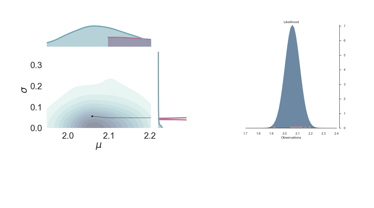
# plot the prior
p1 = pp.PlotPosterior(data1)

p1.create_figure(figsize=(18, 10), textsize=15, joyplot=False, marginal=True, likelihood=True)
p1.plot_marginal(var_names=['$\mu$', '$\sigma$'],
                 plot_trace=False, credible_interval=.92, kind='kde', group='prior')

p1.plot_normal_likelihood('$\mu$', '$\sigma$', '$y$', iteration=-1, hide_bell=True)

p1.likelihood_axes.set_xlim(1.70, 2.40);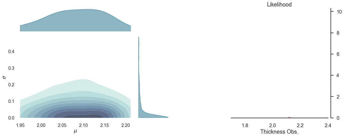

# plot the posterior
def plot_posterior(iteration=-1):
    p1 = pp.PlotPosterior(data1)
    p1.create_figure(figsize=(18, 10), textsize=15, joyplot=False, marginal=True, likelihood=True)
    p1.plot_marginal(var_names=['$\mu$', '$\sigma$'],
                     plot_trace=False, credible_interval=.92, kind='kde', group='both')
    p1.plot_normal_likelihood('$\mu$', '$\sigma$', '$y$', iteration=iteration)
    p1.likelihood_axes.set_xlim(1.70, 2.40);


plot_posterior(-1)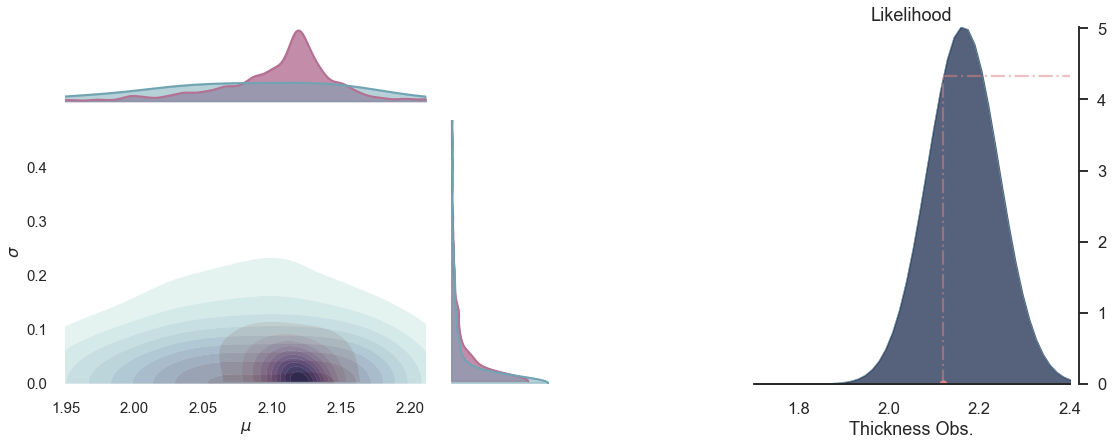

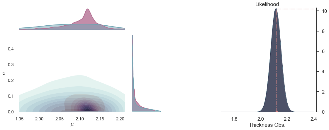
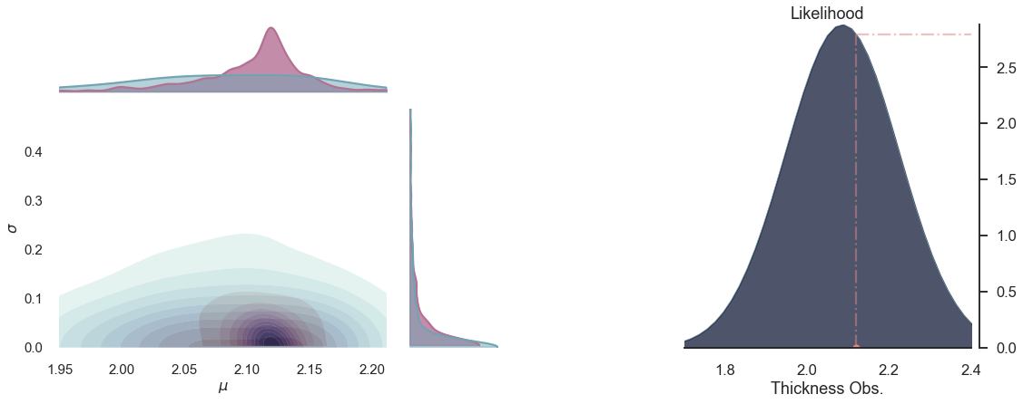
for i in range(5):
    plot_posterior(-i)

MCMC boils down to be a collection of method helping to do bayesian inference, thus based on Bayes Theorem:

P(\theta | x) = \frac{P(x|\theta) P(\theta)}{P(x)}

(2)

$P(\theta | x)$ is the Posterior
$P(x)$ is the Prior
$P(x | \theta)$ is the Likelihood
$P(x)$ the evidence

As calculating the posterior in this form is most likely not possible in real-world problems. If one could sample from the posterior, one might approximate it with Monte Carlo. But in order to sample directly from the posterior, one would need to invert Bayes Theorem.

The solution to this problem is, when we cannot draw MC (in this case Monte Carlo) samples from the distribution directly, we let an MC (now a Markov Chain) do it for us. [1]

What con we do next? Increasing the number of observations - sampling¶

We previously mentioned that we can optimize this model to better fit observations. For this, we generate a prior from the model we previously created, the one with multiple observations from y_obs_list. In the following, samples are iteratively drawn and evaluated to form the posterior. This generates what is called a "trace". A predictive Posterior distribution is then generated from said trace.

# Define model
with pm.Model() as model_multiple_points:
    mu = pm.Normal('$\mu$', 2.08, .07)
    sigma = pm.Gamma('$\sigma$', 0.3, 3)
    y = pm.Normal('$y$', mu, sigma, observed=thickness_observation_list)

# Back to the model with several observations
with model_multiple_points:
    prior = pm.sample_prior_predictive(1000)
    trace = pm.sample(1000, discard_tuned_samples=False, cores=1, chains=1)
    post = pm.sample_posterior_predictive(trace)

# retrieve data
data2 = az.from_pymc3(trace=trace,
                      prior=prior,
                      posterior_predictive=post)

Auto-assigning NUTS sampler...
Initializing NUTS using jitter+adapt_diag...
Sequential sampling (1 chains in 1 job)
NUTS: [$\sigma$, $\mu$]
Sampling chain 0, 0 divergences: 100%|██████████| 1500/1500 [00:00<00:00, 2435.07it/s]
Only one chain was sampled, this makes it impossible to run some convergence checks
100%|██████████| 1500/1500 [00:00<00:00, 2259.04it/s]

Raw observations:¶

The behaviour of this chain is controlled by the observations we fed into the model. Let's have a look again at the observations and how they are spread/distributed:

p2 = pp.PlotPosterior(data2)
p2.create_figure(figsize=(18, 6), joyplot=False, marginal=False)
p2.plot_normal_likelihood('$\mu$', '$\sigma$', '$y$', iteration=-1, hide_bell=True)
p2.likelihood_axes.set_xlabel('Observations')
p2.likelihood_axes.set_xlim(1.90, 2.2)
p2.likelihood_axes.xaxis.set_major_formatter(StrMethodFormatter('{x:,.2f}'))
for tick in p2.likelihood_axes.get_xticklabels():
    tick.set_rotation(45)

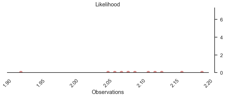
The bulk of observations is between 2.05 and 2.15, one observation at the lower end with 1.92.

Final inference¶

Now let's plot the inferred posterior distribution (i.e. the last sample iteration) and the observations:

p3 = pp.PlotPosterior(data2)
p3.create_figure(figsize=(18, 6), joyplot=False, marginal=False)
p3.plot_normal_likelihood('$\mu$', '$\sigma$', '$y$', iteration=-1, hide_lines=True)
p3.likelihood_axes.set_xlabel('Observations')
p3.likelihood_axes.set_xlim(1.70, 2.40)
p3.likelihood_axes.xaxis.set_major_formatter(StrMethodFormatter('{x:,.2f}'))
for tick in p3.likelihood_axes.get_xticklabels():
    tick.set_rotation(45)

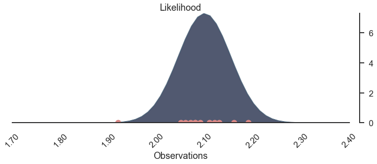
The bell-peak is above a cluster of observations, but the one observation at 1.92 seems to be of greater importance, as otherwise, the highest likelihood might be located more around 2.1.

Joyplot¶

Just plotting the posterior does not convey the underlying process. Attached to GemPy, and used for its stochastic capabilities, visualization methods for drawing distributions were written. More specifically, we use joyplots for showing the change of the distribution (more precisely its mean and its standard deviation) with the progressing chaing:

reload(pp)
joy = pp.PlotPosterior(data2)

joy.create_figure(figsize=(9, 9), joyplot=True, marginal=False,
                  likelihood=False, n_samples=10)
joy.plot_joy(('$\mu$', '$\sigma$'), '$y$', iteration=0);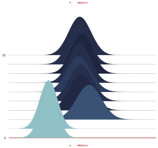

Below we show a gif of how the curve actually moves ( $\mu$ is changed) and changes its width (change in $\sigma$ parameters) with progressive sampling. Dark colors represent an increase in likeliness. However, we see that the colors change with new iterations. That means, that what previously seemed likely becomes less likely as we keep exploring the probability space.

Join probability¶

reload(pp)
p23 = pp.PlotPosterior(data2)

p23.create_figure(figsize=(18, 10), textsize=15, joyplot=False, marginal=True, likelihood=True)
p23.plot_marginal(var_names=['$\mu$', '$\sigma$'],
                  plot_trace=False, credible_interval=.93, kind='kde')

p23.plot_normal_likelihood('$\mu$', '$\sigma$', '$y$', iteration=-1, hide_lines=True)
p23.likelihood_axes.set_xlim(1.70, 2.40);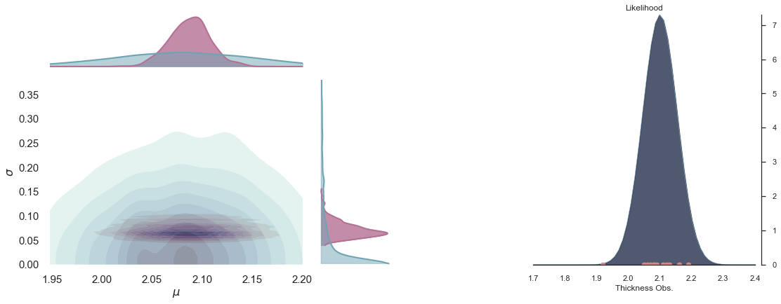

The small gif below shows the first 100 samplings (starting from the 10th iteration) of the chain:

A sped-up version of the full sampling (each 10 steps until we reach the 1000th iteration) provides an impression how we arrive at the posterior distribution...and that the change after the first couple of iterations gets smaller and smaller, as the chain itself gets more and more "educated" about its guesses:

Full plot¶

p3 = pp.PlotPosterior(data2)
p3.create_figure(figsize=(15, 13), joyplot=True, marginal=True, likelihood=True, n_samples=19)
p3.plot_posterior(['$\mu$', '$\sigma$'], ['$\mu$', '$\sigma$'], '$y$', 5,
                  marginal_kwargs={'plot_trace': True, 'credible_interval': .93, 'kind': 'kde'})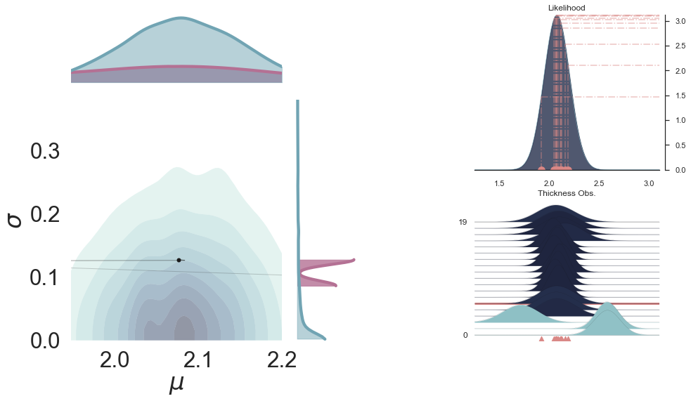

Extending the Dimensions¶

In the model/example before, we had mean and standard deviation of a parameter $y$ , which all were uncertain. Let's take this a step further and say, we look at a layered sequence, so we have a top contact y_top, a bottom contact y_bottom and a resulting thickness y.

thickness_observation = [2.12]
thickness_observation_list = [2.12, 2.06, 2.08, 2.05, 2.08, 2.09,
                              2.19, 2.07, 2.16, 2.11, 2.13, 1.92]

np.random.seed(4003)

After defining some observations (yeah they might be small for layer coordinates, but just think of them as "decameters"), let's set up the model. Now, we actually have three "groups" of probabilistic models, one for each contact and one for the thickness. And on top, mean and standard deviation of contacts and thickness are also distributions:

with pm.Model() as model_layers:
    mu_top = pm.Normal('$\mu_{top}$', 3.05, .2)
    sigma_top = pm.Gamma('$\sigma_{top}$', 0.3, 3)
    y_top = pm.Normal('y_{top}', mu=mu_top, sd=sigma_top, observed=[3.02])

    mu_bottom = pm.Normal('$\mu_{bottom}$', 1.02, .2)
    sigma_bottom = pm.Gamma('$\sigma_{bottom}$', 0.3, 3)
    y_bottom = pm.Normal('y_{bottom}', mu=mu_bottom, sd=sigma_bottom, observed=[1.02])

    mu_thick = pm.Deterministic('$\mu_{thickness}$', mu_top - mu_bottom)
    sigma_thick = pm.Gamma('$\sigma_{thickness}$', 0.3, 3)
    y = pm.Normal('y_{thickness}', mu=mu_thick, sd=sigma_thick, observed=thickness_observation_list)

This yields a suddenly more complex graph:

pm.model_to_graphviz(model_layers)

Now, let's sample from the model:

with model_layers:
    prior = pm.sample_prior_predictive(500)
    trace = pm.sample(500, discard_tuned_samples=False, chains=1, cores=1)
    post = pm.sample_posterior_predictive(trace)

Auto-assigning NUTS sampler...
Initializing NUTS using jitter+adapt_diag...
Sequential sampling (1 chains in 1 job)
NUTS: [$\sigma_{thickness}$, $\sigma_{bottom}$, $\mu_{bottom}$, $\sigma_{top}$, $\mu_{top}$]
Sampling chain 0, 40 divergences: 100%|███████████████████████████████████████████| 1000/1000 [00:03<00:00, 325.95it/s]
There were 40 divergences after tuning. Increase `target_accept` or reparameterize.
Only one chain was sampled, this makes it impossible to run some convergence checks
100%|█████████████████████████████████████████████████████████████████████████████| 1000/1000 [00:02<00:00, 389.98it/s]

data = az.from_pymc3(trace=trace,
                     prior=prior,
                     posterior_predictive=post)

az.plot_density([data, data.prior], shade=.9, data_labels=["Posterior", "Prior"],
                var_names=[
                    '$\\mu_{top}$',
                    '$\\mu_{bottom}$',
                    '$\\mu_{thickness}$',
                    '$\\sigma_{top}$',
                    '$\\sigma_{bottom}$',
                    '$\\sigma_{thickness}$'
                ], colors=[default_red, default_blue]);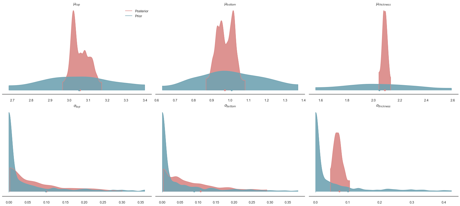

Can we see a correlation between the posteriors of $\mu_{bottom}$ and $\mu_{top}$ ?

p3 = pp.PlotPosterior(data)

p3.create_figure(figsize=(15, 13), joyplot=False, marginal=True, likelihood=False)
p3.plot_marginal(var_names=['$\\mu_{top}$', '$\\mu_{bottom}$'],
                 plot_trace=False, credible_interval=.70, kind='kde'
                 );

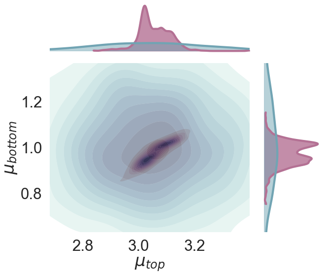
How did we get to this plot? Let's observe the Markov Chain a bit, doing its sampling:

% matplotlib notebook
from importlib import reload

reload(pp)
p3 = pp.PlotPosterior(data)
p3.create_figure(figsize=(15, 9), joyplot=True)


def change_iteration(iteration):
    p3.plot_posterior(['$\\mu_{top}$', '$\\mu_{bottom}$'],
                      ['$\mu_{thickness}$', '$\sigma_{thickness}$'],
                      'y_{thickness}', iteration, marginal_kwargs={"credible_interval": 0.94})


from ipywidgets import interact, interactive, fixed, interact_manual
import ipywidgets as widgets

interact(change_iteration, iteration=widgets.IntSlider(min=0, max=100, step=1, value=10, continuous_update=False));

Applying this to geological modeling¶

In the previous example we assume constant thickness to be able to reduce the problem to one dimension. This keeps the probabilistic model fairly simple since we do not need to deel with complex geometric structures. Unfortunaly, geology is all about dealing with complex three dimensional structures. In the moment data spread across the physical space, the probabilistic model will have to expand to relate data from different locations. In other words, the model will need to include either interpolations, regressions or some other sort of spatial functions. In this paper, we use an advance universal co-kriging interpolator. Further implications of using this method will be discuss below but for this lets treat is a simple spatial interpolation in order to keep the focus on the constraction of the probabilistic model.

# Set up gempy model

# create new model
geo_model = gp.create_model('2-layers')
gp.init_data(geo_model, extent=[0, 12e3, -2e3, 2e3, 0, 4e3], resolution=[100, 1, 100])

# Define formations
geo_model.add_surfaces('surface 1')
geo_model.add_surfaces('surface 2')
geo_model.add_surfaces('basement')

# Map values to formations
dz = geo_model.grid.regular_grid.dz  # this is the thickness of a cell
geo_model.add_surface_values([dz, 0, 0], 'dz')
geo_model.add_surface_values([2.6, 2.4, 3.2], 'density')

# Add geometric input 
geo_model.add_surface_points(3e3, 0, 3.05e3, 'surface 1')
geo_model.add_surface_points(9e3, 0, 3.05e3, 'surface 1')

geo_model.add_surface_points(3e3, 0, 1.02e3, 'surface 2')
geo_model.add_surface_points(9e3, 0, 1.02e3, 'surface 2')

geo_model.add_orientations(6e3, 0, 4e3, 'surface 1', [0, 0, 1])

# Set gravity device
device_loc = np.array([[6e3, 0, 4e3]])
geo_model.set_centered_grid(device_loc, radius=4000, resolution=[10, 10, 30])

# Compile mode
gp.set_interpolator(geo_model,
                    output=['gravity'], pos_density=2,
                    gradient=False,
                    theano_optimizer='fast_run')

Active grids: ['regular']
Active grids: ['regular' 'centered']
Setting kriging parameters to their default values.
Compiling theano function...
Level of Optimization:  fast_run
Device:  cpu
Precision:  float64
Number of faults:  0
Compilation Done!
Kriging values: 
                          values
range              13266.499161
$C_o$            4190476.190476
drift equations             [3]

<gempy.core.interpolator.InterpolatorModel at 0x12f3f24eb80>

Plotting input of model¶

p3 = gp.plot.plot_2d(geo_model, show_data=True, show_results=False, figsize=(18, 10))  #plot_data(geo_model)
p3.fig.set_figwidth(20)
p3.fig.axes[-1].scatter([3e3], [4e3], marker='^', s=200, c='k', zorder=10)
p3.fig.axes[-1].scatter([9e3], [4e3], marker='^', s=200, c='k', zorder=10)
p3.fig.axes[-1].scatter([6e3], [4e3], marker='x', s=400, c='red', zorder=10)

p3.fig.axes[-1].vlines(3e3, .5e3, 10e3, linewidth=4, color='gray', )
p3.fig.axes[-1].vlines(9e3, .5e3, 10e3, linewidth=4, color='gray')
p3.fig.axes[-1].vlines(3e3, .5e3, 10e3)
p3.fig.axes[-1].vlines(9e3, .5e3, 10e3)
p3.fig.axes[-1].vlines(9e3, .5e3, 10e3)
p3.fig.axes[-1].fill_between(x=[5.5e3, 6.5e3], y1=[0, 0], y2=[10e3, 10e3], alpha=.7, color=default_blue);

gp.plot_2d(geo_model, direction='z', figsize=(18, 10))
plt.scatter(device_loc[:, 0], device_loc[:, 1], s=300, marker='x', c='r')

<matplotlib.collections.PathCollection at 0x12f47b0f520>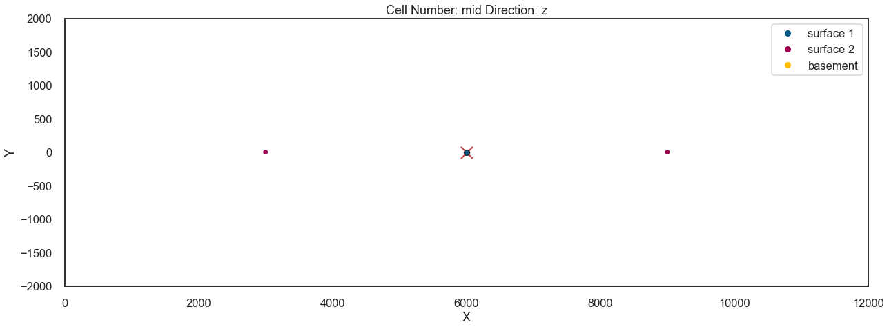

Interpolating¶

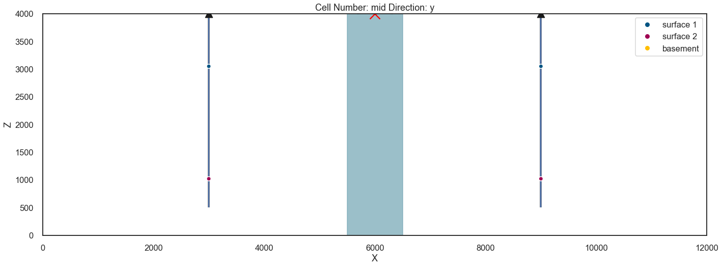
sol = gp.compute_model(geo_model, set_solutions=True, compute_mesh=False)

p3 = gp.plot_2d(geo_model, cell_number=0, show_data=True, direction='y')
p3.fig.set_figwidth(20)
p3.fig.axes[-1].scatter([3e3], [3.9e3], marker='^', s=200, c='k', zorder=10)
p3.fig.axes[-1].scatter([9e3], [3.9e3], marker='^', s=200, c='k', zorder=10)
p3.fig.axes[-1].scatter([6e3], [4e3], marker='x', s=400, c='red', zorder=10)

p3.fig.axes[-1].vlines(3e3, .5e3, 10e3, linewidth=4, color='gray', )
p3.fig.axes[-1].vlines(9e3, .5e3, 10e3, linewidth=4, color='gray')
p3.fig.axes[-1].vlines(3e3, .5e3, 10e3)
p3.fig.axes[-1].vlines(9e3, .5e3, 10e3)
p3.fig.axes[-1].vlines(9e3, .5e3, 10e3)
p3.fig.axes[-1].fill_between(x=[5.5e3, 6.5e3], y1=[0, 0], y2=[10e3, 10e3], alpha=.7, color=default_blue);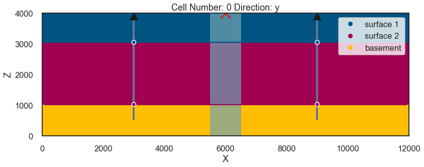

geo_model.solutions.fw_gravity

array([-352.65902036])

geo_model.solutions.block_matrix[0][1].reshape(100, 1, 100)[25, 0, :].sum()

960.0

import matplotlib.pyplot as plt
plt.imshow(geo_model.solutions.block_matrix[0][1].reshape(100, 1, 100)[:, 0, :])

<matplotlib.image.AxesImage at 0x12f4b86e0a0>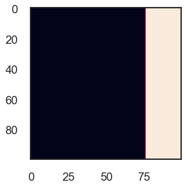

# Reset
grav__ = []

def plot_section(z1, z2):
    geo_model.modify_surface_points([2, 3], Z=z1)
    geo_model.modify_surface_points([0, 1], Z=z2)
    gp.compute_model(geo_model, output='gravity', compute_mesh=False)
    grav__.append(geo_model.solutions.fw_gravity)
    print(grav__)
    fig = gp.plot_2d(geo_model, cell_number=0, show_data=True, direction='y')
    plt.scatter(geo_model.grid.centered_grid.values[:, 0], geo_model.grid.centered_grid.values[:, 2],
                c='k', s=3)
    plt.show()
    plt.plot(grav__, 'o')
    plt.ylabel('grav')
    plt.show()
    return fig

%matplotlib notebook
from ipywidgets import interact, interactive, fixed, interact_manual
import ipywidgets as widgets

interact(plot_section,
         z1=widgets.IntSlider(min=2.7e3, max=3.5e3, step=100, continuous_update=False),
         z2=widgets.IntSlider(min=.8e3, max=1.6e3, step=100, continuous_update=False))

Bayesian Inference with GemPy and Pymc3¶

indices_bool = geo_model.surface_points.df['surface'].isin(['surface 1', 'surface 2'])
indices = geo_model.surface_points.df.index[indices_bool]
Z_init = geo_model.surface_points.df.loc[indices, 'Z'].copy()

import theano.tensor as tt


def compute_gempy_model(Z_pos):
    geo_model.modify_surface_points(indices, Z=Z_pos)
    gp.compute_model(geo_model)


def sample_grav(Z_var2):
    compute_gempy_model(Z_var2)

    # Returns the 3d lith array
    return geo_model.solutions.fw_gravity


def sample_lith(Z_var):
    compute_gempy_model(Z_var)
    return geo_model.solutions.block_matrix[0][1]


class GemPyGrav(tt.Op):
    itypes = [tt.dvector]
    otypes = [tt.dvector]

    def perform(self, node, inputs, outputs):
        theta, = inputs
        mu = sample_grav(theta)
        outputs[0][0] = np.array(mu)


class GemPyLith(tt.Op):
    itypes = [tt.dvector]
    otypes = [tt.dvector]

    def perform(self, node, inputs, outputs):
        theta, = inputs
   
        mu = sample_lith(theta)
        outputs[0][0] = np.array(mu)


gempy_grav = GemPyGrav()
gempy_lith = GemPyLith()

gravity_observations = 1e3 * np.array([-0.34558686, -0.3648658,
                                       -0.3448658, -0.3663401,
                                       -0.3441554, -0.3634569,
                                       -0.3472901, -0.36575098,
                                       -0.35575098, -0.36424498,
                                       -0.35643718], dtype='float64')

thickness_obs = 1e3 * np.array([1.32, 1.16, 1.28, 1.25, 1.08, 1.09,
                                1.19, 0.87, 0.96, 0.31, 0.83, 0.92])

with pm.Model() as model:
    Z_var = pm.Normal('depths', Z_init, 200 , shape=4, dtype='float64')

    grav = gempy_grav(Z_var)
    geo = gempy_lith(Z_var)

    grav = pm.Deterministic('gravity', grav[0])
    well_1 = geo.reshape((100, 1, 100))[25, 0, :]
    well_2 = geo.reshape((100, 1, 100))[75, 0, :]

    thick_1 = pm.Deterministic('thick_1', well_1.sum())
    thick_2 = pm.Deterministic('thick_2', well_2.sum())

    sigma_grav = pm.Normal('sigma', mu=2500, sigma=1500)
    sigma_thick = pm.Gamma('sigma_thickness', mu=3000, sigma=3000)
    sigma_thick2 = pm.Gamma('sigma2_thickness', mu=3000, sigma=3000)

    obs_grav = pm.Normal('y', mu=grav, sd=sigma_grav, observed=gravity_observations)
    obs_thick_1 = pm.Normal('y2', mu=thick_1, sd=sigma_thick, observed=thickness_obs)
    obs_thick_2 = pm.Normal('y3', mu=thick_2, sd=sigma_thick2, observed=thickness_obs)

with model:
    prior = pm.sample_prior_predictive(100)

data = az.from_pymc3(prior=prior)
az.plot_density([data.prior], shade=.9, data_labels=["Prior"],
                var_names=['depths', 'gravity', 'thick_1', 'thick_2']);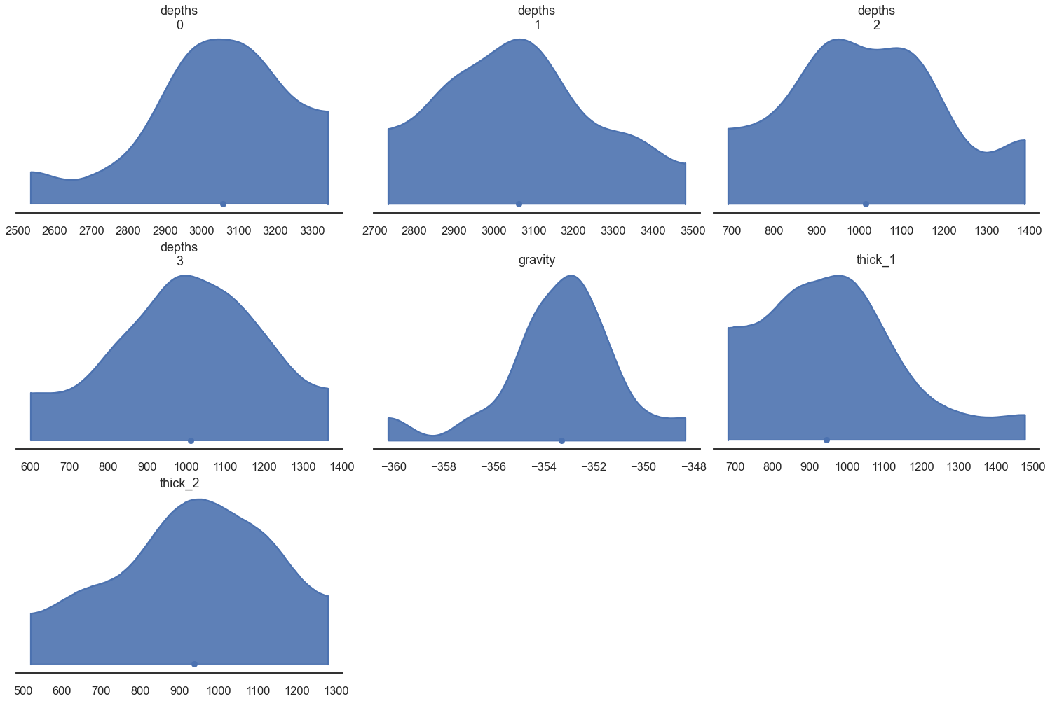

with model:
    trace = pm.sample(2000, cores=1, chains=1, step=pm.Metropolis(tune_interval=100), tune=500)

Sequential sampling (1 chains in 1 job)
CompoundStep
>Metropolis: [sigma2_thickness]
>Metropolis: [sigma_thickness]
>Metropolis: [sigma]
>Metropolis: [depths]
Sampling chain 0, 0 divergences: 100%|██████████| 2500/2500 [17:56<00:00,  2.32it/s]  
Only one chain was sampled, this makes it impossible to run some convergence checks

with model:
    post = pm.sample_posterior_predictive(trace)

100%|██████████| 2000/2000 [02:45<00:00, 12.06it/s]

data = az.from_pymc3(trace=trace,
                     prior=prior,
                     posterior_predictive=post)

az.plot_density([ data.prior, data], shade=.9, data_labels=[ "Prior", "Posterior"],
                var_names=['depths', 'gravity', 'thick_1', 'thick_2']);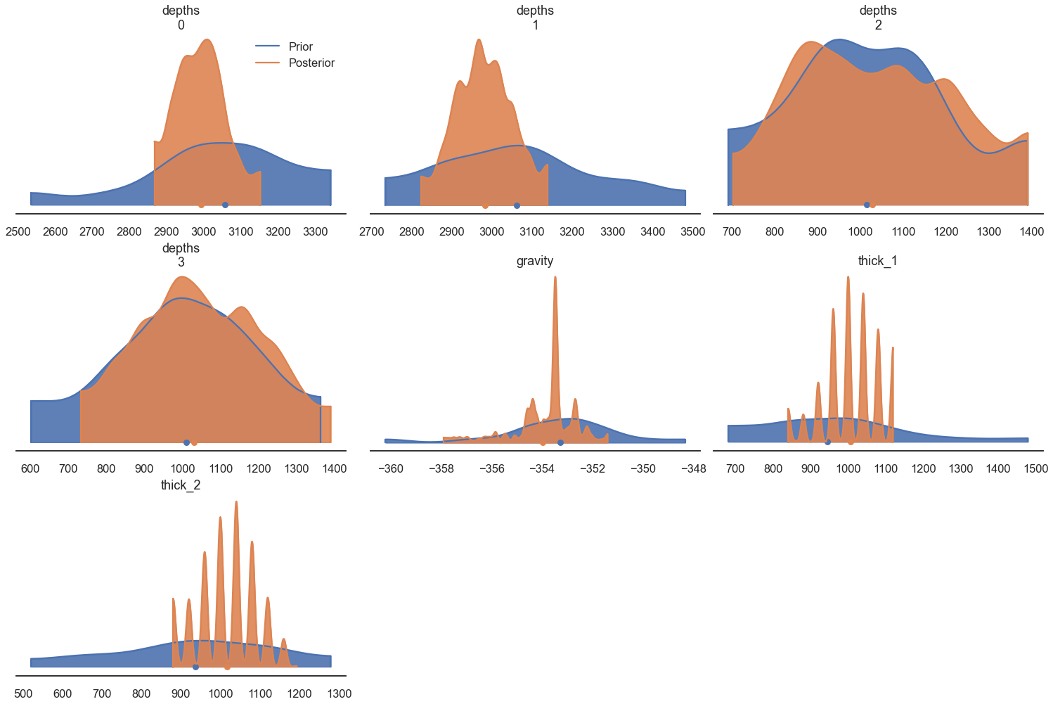

References¶

[1] Thomas Wiecki 2015. MCMC sampling for dummies https://twiecki.io/blog/2015/11/10/mcmc-sampling/ (last visited 2022-04-18)
[2] Gallagher, K., Charvin, K., Nielsen, S., Sambridge, M., & Stephenson, J. (2009). Markov chain Monte Carlo (MCMC) sampling methods to determine optimal models, model resolution and model choice for Earth Science problems. Marine and Petroleum Geology, 26(4), 525-535.
[3] Salvatier, J., Wiecki, T. V., & Fonnesbeck, C. (2016). Probabilistic programming in Python using PyMC3. PeerJ Computer Science, 2, e55.

T22 - What is Markov chain Monte Carlo

Basic Introduction - Who is Markov and what do they do in Monte Carlo?