Machine learning models for Geoscience
In this tutorial, we’ll run a fairly basic random forest prospectivity analysis workflow applied to tin-tungsten (Sn-W) deposits in northeastern Tasmania.
We'll use open data sets provided by Mineral Resources Tasmania and Geoscience Australia, all of which are available to download from our public Google Drive. The roadmap for the tutorial is as follows:
- Load and inspect data sets
- mineral occurrence point data sets with geopandas
- gravity, magnetic and radiometric data sets with rasterio
- Combine data sets to build a labeled Npixel, Nlayers array for model training
- inspect differences between proximal vs. distal to mineralisation pixels
- Train a random forest classifier and apply to all pixels, visualise results
- evaluate performance with a randomly selected testing subset
- repeat with stratified classes
- Develop a checkerboard data selection procedure, train and evaluate models
- discuss effects of spatially separated testing data
- Investigate occurrence holdout models with a spatially clustered approach
Instructors
- Thomas Ostersen - Datarock Applied Science
- Tom Carmichael - Datarock Applied Science
Prerequisites
- Knowledge of Python is assumed and all coding will be done within a Jupyter notebook
- We'll use numpy for data handling and matplotlib for data visualisation
- Point data sets are handled with geopandas, a pandas-like library for vector GIS processing
- Rasterio is used to read and write gridded raster data sets
- The scikit-learn implementation of the random forest algorithm is used for all modelling
- Class stratification in modelling procedures use the imbalanced-learn library
Setup
There are a few things you'll need to follow the tutorial:
- A working Python installation (Anaconda or Miniconda)
- The Geospatial ML tutorial conda environment installed
- A web browser that works with Jupyter notebooks (basically anything except Internet Explorer)
To get things setup, please do the following.
Windows users: When you see "terminal" in the instructions, this means the "Anaconda Prompt" program for you.
Step 1
Install a Python distribution:
In this tutorial we will be using the Anaconda Python distribution along with the conda package manager. If you already have Anaconda or Miniconda installed, you can skip this step.
If not, please follow Matt Hall's video tutorial from Transform2020: youtube instructions
Step 2
Create the t22-mon-ml-models conda environment:
- Download the
environment.ymlfile from here (right-click and select "Save page as" or similar) - Make sure that the file is called
environment.yml. Windows sometimes adds a.txtto the end, which you should remove - Open a terminal (Anaconda Prompt if you are running Windows). The following steps should be done in the terminal
- Navigate to the folder that has the downloaded environment file
- Create the conda environment by running
conda env create --file environment.yml(this will download and install all of the packages used in the tutorial)
Step 3
- Download the zipped data set from our public Google drive, this should look like the following screenshot
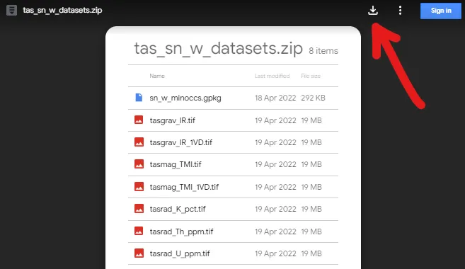
- Once downloaded, unzip the data set and copy it to your working directory of choice
Step 4
Start JupyterLab:
- Windows users: Make sure you set a default browser that is not Internet Explorer.
- Activate the conda environment:
conda activate t22-mon-ml-models - Start the JupyterLab server:
jupyter lab - Jupyter should open in your default web browser. We'll start from here in the tutorial and create a new notebook together.
IF EVERYTHING ELSE FAILS
If you really can't get things to work on your computer, you can run the code online through Google Colab (you will need a Google account). A starter notebook that installs all the tutorial dependencies and downloads the tutorial data can be found here:
https://colab.research.google.com/drive/1jAW8A4hDdFn4An3I3jtVJiTxzNn08oRU?usp=sharing
To save a copy of the Colab notebook to your own account, click on the "Open in playground mode" and then "Save to Drive". You might be interested in this tutorial for an overview of Google Colab.
Data License
All data presented in this tutorial were derived from open data sets made available through Mineral Resources Tasmania and Geoscience Australia.
LICENCE CONDITIONS
By exporting this data you accept and comply with the terms and conditions set out below:
Creative Commons Attribution 3.0 Australia
You are free to:
- Share — copy and redistribute the material in any medium or format
- Adapt — remix, transform, and build upon the material for any purpose, even commercially.
Under the following terms:
- Attribution — You must give appropriate credit, provide a link to the license, and indicate if changes were made. You may do so in any reasonable manner, but not in any way that suggests the licensor endorses you or your use. “
Acknowledgments
This tutorial borrowed HEAVILY from Santiago Soler, Andrea Balza Morales and Agustina Pesce's superb Harmonica tutorial from Transform2021, also documented on github here: https://github.com/fatiando/transform21.