First a quick tour of the jupyter notebook¶

Shortcuts
Getting help
Cell types
Executing cells

Formatted text¶

We can write formated text in Markdown cells (Esc + m) and there are plenty of resources available:

The original Markdown page by John Gruber: daringfireball.net/projects/markdown
Getting started with markdown: markdownguide.org/getting-started
Cheat sheet: markdownguide.org/cheat-sheet

H4-heading¶

Unordered list

item 1
item 2
- sub-item a
- sub-item b
item 3

Ordered list

first
second
third

italic, bold, underline (not strictly markdown but works in the notebook)

quoted text

Syntax	Description
Header	Title
Paragraph	Text

Equations¶

Mathematical expressions in notebooks use LaTeX: overleaf.com/learn/latex/Mathematical_expressions

Inline Gardner's equation $\rho = \alpha {V_P}^{\beta}$

Centered equation Darcy'y Law

q = -\frac{k}{\mu L} \Delta p

(1)

Code¶

in-line code

and multiline formatted code:

# Some formatted python code

def say_hi():
    """Just print hello!"""
    print('Hello!')
    return None

Code output¶

print('Hello Transfrom 2022!')

Hello Transfrom 2022!

Images¶

A gentle introduction to python¶

Things you already know¶

mathematical operators¶

# Live coding of basic mathematical operators

# Press shift+enter to execute a cell
2 + 3

5

2 + 3.5

5.5

15.5 - 76

-60.5

45 * 0.4

18.0

23 / 2

11.5

# Long division
23 // 2

11

# Remainder of long division: the "modulo operator"
23 % 2

1

2**3

8

logical operators¶

# Live coding of logical operators

23 > 4

True

534 < 100

False

100 <= 100

True

200 >= 199

True

13 == 15

False

43 != 49

True

# Combining them
11 % 2 == 0

False

(4 > 2) and (50 <= 10)

False

(4 > 2) or (50 <= 10)

True

Assignment¶

x = 10
# no output!

10

Stepping sideways out of your comfort zone¶

Words and collections in python (i.e. str, list, dict)

`str`¶

word = 'python'
type(word)

str

word

'python'

# single vs double quotes

double_quotes = "same thing"
double_quotes

'same thing'

len(word)

6

# str methods

word.upper()

'PYTHON'

word

'python'

`list`¶

word_list = ['python', 'geology', 'programming', 'code', 'outcrop']
# again, no output, assignment is silent

# exploring lists

type(word_list)

list

len(word_list)

5

word_list

['python', 'geology', 'programming', 'code', 'outcrop']

'geology' in word_list

True

word_list.append('mineral')
# no output

word_list

['python', 'geology', 'programming', 'code', 'outcrop', 'mineral']

Indexing and slicing¶

We can reach into these collections, there are two main things to remember:

python starts counting at 0
we use square brackets []

Indexing and slicing `str`¶

len(word)

6

word

'python'

word[0]

'p'

word[5]

'n'

# half-open interval
word[0:3]

'pyt'

Indexing and slicing `list`¶

# same thing with `list`
word_list

['python', 'geology', 'programming', 'code', 'outcrop', 'mineral']

word_list[0]

'python'

word_list[-1]

'mineral'

word_list[4:]

['outcrop', 'mineral']

`dict`¶

container = {'words': word_list, 'word': word, 'transform': 2022}
container

{'words': ['python', 'geology', 'programming', 'code', 'outcrop', 'mineral'],
 'word': 'python',
 'transform': 2022}

# Exploring python dict

container.keys()

dict_keys(['words', 'word', 'transform'])

container.values()

dict_values([['python', 'geology', 'programming', 'code', 'outcrop', 'mineral'], 'python', 2022])

container.get('word')

'python'

Importing more functions¶

Sometimes we need to reach for some part of python that isn't loaded by default, there are three major ways to import packages:

import package -> imports everything. Access things using package.function().
import package as pkg -> imports everything with an alias. Accessing things using pkg.function().
from package import function1, function2 -> import only function1 and function2. Accessed as function1() and function2().

Here we use the third method to import the datetime object from the datetime library:

from datetime import datetime

And we can now update the dict with a new value, for example today's date using the datetime object we just imported:

# using datetime to add today's date to the dict

# Build this up
container.update({'Location': 'Global', 'date': datetime.now().date().isoformat()})

container

{'words': ['python', 'geology', 'programming', 'code', 'outcrop', 'mineral'],
 'word': 'python',
 'transform': 2022,
 'Location': 'Global',
 'date': '2022-04-07'}

container['date']

'2022-04-07'

Keying into a `dict`¶

container.keys()

dict_keys(['words', 'word', 'transform', 'Location', 'date'])

container.get('word')

'python'

container['word']

'python'

Controlling the flow¶

if ... else

We often want to make decision in our code based on conditions, so first we need a bool-ean condition:

x < 5

False

word == 'python'

True

42 % 2 == 0

True

'Global' in container.values()

True

container['words'][1] == 'geology'

True

Now we can use these in the basic if statement:

if word == 'python':
    print('Code!')

Code!

Let's look at container.values() again:

container.values()

dict_values([['python', 'geology', 'programming', 'code', 'outcrop', 'mineral'], 'python', 2022, 'Global', '2022-04-07'])

And we can check for membership of this container.values():

'Global' in container.values()

True

So now we can use this in our conditional statement:

if 'python' in container.values():
    print('Code!')
else:
    print('No code.')

Code!

What does this look like with a geological example?

porosity = 0.23

if porosity >= 0.3:
    reservoir = 'Good'
elif 0.15 < porosity < 0.3:
    reservoir = 'Medium'
else:
    reservoir = 'Poor'

reservoir

'Medium'

Say that again?¶

loops in python (for, list comprehensions)

One of the main advantages of computers is the ability to repeat tedious tasks efficiently. Let us first load some data, we will use numpy for this:

import numpy as np

data = np.load('./data/GR-NPHI-RHOB-DT.npy')
print(data.shape)
nphi = data[:,1]
print(nphi.shape)

(71, 4)
(71,)

nphi

array([0.2455, 0.2432, 0.2406, 0.2393, 0.2416, 0.2294, 0.2516, 0.2543,
       0.2299, 0.2547, 0.2708, 0.2583, 0.237 , 0.2541, 0.2331, 0.2469,
       0.2529, 0.2341, 0.2251, 0.2293, 0.2193, 0.2134, 0.2422, 0.2436,
       0.2024, 0.2314, 0.2373, 0.2112, 0.2358, 0.2278, 0.205 , 0.2283,
       0.2436, 0.1864, 0.2222, 0.2115, 0.2033, 0.2279, 0.1988, 0.2214,
       0.2361, 0.2339, 0.2301, 0.226 , 0.2365, 0.2512, 0.2186, 0.2294,
       0.2348, 0.2416, 0.2434, 0.2178, 0.2229, 0.2185, 0.2268, 0.2256,
       0.2155, 0.2351, 0.2216, 0.2042, 0.2133, 0.2411, 0.221 , 0.2219,
       0.22  , 0.2361, 0.2378, 0.2233, 0.2122, 0.2439, 0.2273])

for porosity in nphi[:5]: # !! we only use the first 5 porosities to test our code (using a slice)
    print(porosity)

0.24550000004046355
0.2432000000221169
0.2405999999336257
0.2392999999883031
0.24160000002507376

import matplotlib.pyplot as plt
plt.plot(nphi)
plt.hlines(0.24, 0, 70, color='r')
plt.hlines(0.22, 0, 70, color='r')
plt.ylabel('NPHI')
plt.xlabel('Sample number')
plt.grid(alpha=0.4)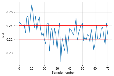

porosity = 0.23

if porosity >= 0.24:
    reservoir = 'Good'
elif 0.22 < porosity < 0.24:
    reservoir = 'Medium'
else:
    reservoir = 'Poor'

reservoir

'Medium'

for porosity in nphi[:5]:
    if porosity >= 0.24:
        reservoir = 'Good'
    elif 0.22 < porosity < 0.24:
        reservoir = 'Medium'
    else:
        reservoir = 'Poor'
    print(reservoir)

Good
Good
Good
Medium
Good

good_reservoir_count = 0

for porosity in nphi[:10]:
    if porosity >= 0.24:
        good_reservoir_count += 1

good_reservoir_count

7

good_reservoir_count = 0

for porosity in nphi:
    if porosity >= 0.24:
        good_reservoir_count += 1

good_reservoir_count

20

# IGNORE this if it's too much of a stretch!
good_resevoir_lc = sum([1 for poro in nphi if poro > 0.24])
good_resevoir_lc

20

An image speaks a thousand words¶

The python-visualization-landscape is vast and can be intimidating, no doubt you'll see many great examples during Transform 2022, but the place to start is usually matplotlib, you can reach the docs directly from with the jupyter notebook:

import matplotlib.pyplot as plt

plt.plot(nphi)

[<matplotlib.lines.Line2D at 0x7f4e835d4d00>]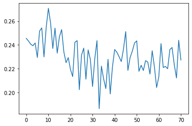

plt.plot(nphi, 'o-', c='g')

[<matplotlib.lines.Line2D at 0x7f4e836a21f0>]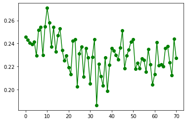

fig, ax = plt.subplots()

ax.plot(nphi, 'o-', c='g', lw=0.4, markersize=2)
ax.set_ylabel('NPHI')
ax.set_xlabel('Sample number')
ax.set_title('Simple Porosity plot')
ax.grid(alpha=0.4)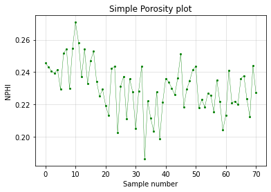

Now we have created a plot, let's pull all of this together a single cell and save the figure:

import numpy as np
import matplotlib.pyplot as plt


data = np.load('./data/GR-NPHI-RHOB-DT.npy')
nphi = data[:,1]

fig, ax = plt.subplots()

ax.plot(nphi, 'o-', c='g', lw=0.4, markersize=2)
ax.set_ylabel('NPHI')
ax.set_xlabel('Sample number')
ax.set_title('Simple Porosity plot')
ax.grid(alpha=0.4)

plt.savefig('./images/NPHI_plot.png')

plt.show()

Interactive plots¶

It is possible to add interactivity to plots in the Jupyter notebook using ipywidgets, without going through a full tutorial, here is a simple demo extending the plot we've been working with:

from ipywidgets import interact
import ipywidgets as widgets


@interact(high=widgets.FloatSlider(value=0.24, min=0.22, max=0.28, step=0.001, continuous_update=False),
          low=widgets.FloatSlider(value=0.22, min=0.18, max=0.22, step=0.001, continuous_update=False)
         )
def poro_high_low(high, low):
    """Create an interactive plot with ipywidgets."""
    fig, ax = plt.subplots(figsize=(14, 6))
    ax.plot(nphi, c='k', lw=1, markersize=6)
    ax.plot(np.where(nphi > high, nphi, None), '^', c='r', lw=0.4, markersize=10)
    ax.plot(np.where((nphi < high) & (nphi > low), nphi, None), 'o', c='g', lw=0.4, markersize=8)
    ax.plot(np.where(nphi < low, nphi, None), 'v', c='b', lw=0.4, markersize=8)
    ax.fill_between(np.arange(nphi.size), low, high, color='g', alpha=0.1)
    ax.set_ylabel('NPHI')
    ax.set_xlabel('Sample number')
    ax.set_title('Simple Porosity plot')
    ax.axhline(high, ls='--' ,c='r', label='high')
    ax.axhline(low, ls='-.', c='b', label='low')
    ax.legend()
    ax.grid(alpha=0.4)
    
    return None

Wrap it up and do it again¶

Part of the beauty of code is its reusabilty, we've used functions already:

type(print)

builtin_function_or_method

sum([1, 2, 3])

6

# using plt.scatter

xs = [1, 2, 3, 4, 5, 6, 7, 8, 9, 10]
x2 = [x**2 for x in xs]
plt.scatter(xs, x2, c='r')

<matplotlib.collections.PathCollection at 0x7f4e831bf460>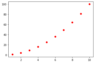

# writing our own simple function

def my_adder(a, b):
    """Add two numbers."""
    return a + b

my_adder?

my_adder(45, 98)

143

Writing actual equations in python¶

Remember this equation?

\rho = \alpha {V_P}^{\beta}

(2)

Let's turn it into a python function:

def gardner(vp, alpha=310, beta=0.25):
    """Evaluate gardner's relation.
    Args:
        vp (float): P-wave velocity
        alpha (float-like): alpha scalar
        beta (float-like): beta exponent
    Returns:
        rho (float): density
    Source: https://subsurfwiki.org/wiki/Gardner%27s_equation
    """
    return alpha * vp**beta

gardner(2766)

2248.147169062099

Where to next?¶

Useful (and approachable) documentation
python.org/tutorial
matplotlib gallery
w3schools/python
Books
Python Crash Course, 2nd Edition
Automate the Boring Stuff with Python, 2nd Edition
Learning Python: Powerful Object-Oriented Programming
Cheatsheets
pythoncheatsheet
Basic cheatseet
Geophysics cheatsheet
Rock physics cheatsheet
Petrophysics cheatsheet
Petroleum cheatsheet
Transform youtube tutorials
Preparing for Transform 2020, setup guides for Windows and Linux
Learning Python for Geoscience, a playlist of setup instructions and tutorials covering introductions to python, python subsurface tools, geospatial analysis, statistics and data analysis and well data exploration.
Transform 2021 all the content from the 2021 edition!
Transform 2020 all the content from the 2020 edition!
Your own awesome project! The best way to learn anything is through practice, so now you should think of a task you perform at work on in your hobbies that you can break down into programmable steps, then code it up in python little by little, and before you know it, you'll be a pythonista!

T22 - Getting started in python

Installation and Setup

Intro to Python

First a quick tour of the jupyter notebook¶

Formatted text¶

H4-heading¶

Equations¶

Code¶

Code output¶

Images¶

A gentle introduction to python¶

Things you already know¶

mathematical operators¶

logical operators¶

Assignment¶

Stepping sideways out of your comfort zone¶

str¶

list¶

Indexing and slicing¶

Indexing and slicing str¶

Indexing and slicing list¶

dict¶

Importing more functions¶

Keying into a dict¶

Controlling the flow¶

Say that again?¶

An image speaks a thousand words¶

Interactive plots¶

Wrap it up and do it again¶

Writing actual equations in python¶

Where to next?¶

`str`¶

`list`¶

Indexing and slicing `str`¶

Indexing and slicing `list`¶

`dict`¶

Keying into a `dict`¶