Latest developments in sensor technology (e.g., satellite, airborne) provide us a large amount of high-quality data, which contains important information about the subsurface properties and processes. The size and complexity of geophysical data that we need to deal with is exponentially increasing. As geoscientists, therefore, data-driven problem solving is an essential skill to explore the flooding of data and extract meaningful information from them. In this lecture, I focus on constructing a mental model for “a data-driven problem solving” with an example in a mining application. The methodology that I am using for the data-driven problem solving in the lecture is an inversion technique, which has been a core framework for geophysicists to image distribution of subsurface physical properties (e.g., seismic velocity, density, electric resistivity, magnetic susceptibility). I start with some important concepts about how we transmit energy into Earth’s subsurface, and measure derived signals including information about the subsurface. Then, I explain how we can formulate a problem in a way which we can drive a solution from the measured data and prior knowledge about the problem.

A motivating example: Raglan Mineral Deposits¶

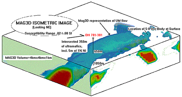
We used a mining case history at Raglan Deposits as a motivating example. About 20 years ago, airborne magnetic surveys were flown, and magnetic data were acquired. This data set was inverted using the MAG3D code developed by UBC-GIF group Li & Oldenburg, 1996, and a 3D susceptibility model was obtained. This was sort of the first time that field magnetic data was inverted in 3D, and made a significant impact on locating drilling location for a mineral exploration. Below image shows the recovered subsurface model (i.e., the distribution of magnetic susceptibility) and the spotted drill hole location by geologists based upon this subsurface model obtained from the airborne geophysical data.

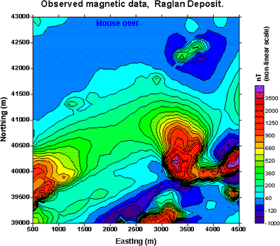
As shown in the above image, the recovered model shows the connected ultramafics containing target minerals (e.g., sulphides), but initially it was thought that there were two separate ultramafic pipes. This was based upon the acquired magnetic data shown below as well as the observed outcrops of the ultramafics around the two distinct anomalies shown in the image.

In this tutorial, we used this historical data set as an example to introduce fundamental concepts about the geophysical inversion, which provides a “data-driven” solution for extracting useful information from geophysical data. Numerical examples used in the tutorial are available through the github repository. Three main Jupyter notebooks used in the tutorial can be viewed in the subsections of this curvenote.

Resources¶

• Transform 2021 conference: https://softwareunderground.org/events/transform-2021
• Tutorial video: http://bit.ly/transform-2021-inversion-for-geologitst-video
• Slides: http://bit.ly/transform-2021-slides
• GitHub: https://github.com/simpeg/transform-2021-simpeg
• Inversion module: https://curvenote.com/@geosci/inversion-module